Namrata Gawande*![]() | Dinesh Goyal
| Dinesh Goyal![]() | Kriti Sankhla
| Kriti Sankhla![]()
© 2025 The authors. This article is published by IIETA and is licensed under the CC BY 4.0 license (http://creativecommons.org/licenses/by/4.0/).
OPEN ACCESS
Chronic heart failure (CHF) detection remains a critical challenge in healthcare due to its complex and multifactorial nature. Heart sound analysis serves an important part in identifying cardiovascular disease; however, the availability of balanced datasets for training machine learning models remains a challenge due to inherent class imbalances. To address this, an inception-based Generative Adversarial Networks (GAN) method is proposed to acquire the distribution of heart sound classes and generate synthetic samples for underrepresented classes. The model is applied to the unbalanced PhysioNet dataset of heart sound signals, and features extracted from real and synthetic data are combined into feature vectors, enabling feature fusion, which are passed to various classification models. This study attempts to fine-tune pre-trained convolutional neural network models, specifically VGG16 and MobileNet for classification of Heart sound signals. The results of proposed models are compared with and without GAN model on heart sound signals and gets significant improvement with KNN Hyper parameter tuning, Proposed Autoencoder + CNN model and Fine-tune MobileNet and VGG16 algorithm. KNN hyperparameter tuning refines the model’s decision boundaries for better classification accuracy, while the Autoencoder + CNN architecture leverages deep feature learning to extract high-level representations, enhancing diagnostic precision. The model outperforms machine learning and deep learning models, improving overall recall and F1-score by approximately 8%.
phonocardiograms, heart sound classification generative adversarial network, deep learning, transfer learning
The heart is a vital organ, and cardiovascular disease is a global health concern. The World Health Organization reports that heart disorders are the primary reason of death. The globe has approximately 17.3 million fatalities every year [1]. The shortage of medical experts in developing countries exacerbates the situation. Heart computer signals, such as electrocardiograms and PCGs, indicate circulatory system malfunction. Phonocardiograms (PCGs) can show heart valve disease or deformity [2].
A clinician during cardiac auscultation uses a stethoscope to listen for certain sounds to determine the state of the heart. Blood pressure, opening, and closure of the heart valves and contraction of cardiac muscle create a vibration. The vibration travels through the tissues to reach the thorax and is used to detect the heart sound. Murmurs indicate that there is a problem with the heart. These murmurs have been classified as abnormal heart sounds. Murmurs are created as blood flows through the heart system in a turbulent manner. Pitch and timing of the noises are important parameters to detect a problem in the heart. Health practitioners classify heart sounds based on a variety of characteristics, the most prevalent of which are timing, cadence, length, pitch, and form [3]. Figure 1 shows normal and abnormal heart sound signals.
With improved cardiovascular technology, the workload of medical professionals has increased consequently, accurate detection of heart diseases becomes challenging. The approaches that have already been applied in the automatic diagnosis of cardiac problems with minimal clinician intervention include artificial intelligence and deep learning. Such ML methods [4], devoting manual feature extraction and selection, have weaknesses in picking up the right features from patient data. However, DL-based models are more accurate and effective in predicting heart diseases but require computationally intensive training with a large dataset [5, 6].
Classifiers overfit when trained on low-sample datasets, so they fail to attain optimal performance on real-world data [7]. Abnormal heart sounds are less frequent in real-world datasets because there is a lower incidence of cardiac illnesses within the general population. GANs can, therefore, be used to address class imbalances. In this regard, the present study is aimed at developing a GAN-based model for the generation of balanced heart sound data in addressing the case of class imbalance. The proposed model creates synthetic samples through a process similar to actual recordings but guarantees that the normal and abnormal classes will be balanced using the adversarial training framework in GANs.
Transfer learning based pre-trained models such as VGG16 and MobileNet and fine-tuning [8] these models on the balanced dataset allows their learned representations to adapt to the intricacies of heart sound classification. A combination of GAN-generated data, application of pre-trained models, and fine-tuning enables better generalization capacity for heart sound classification models. This will enhance the model on unseen samples by enabling it to learn discriminative features from a wider representation of the data.
Figure 1. Normal and abnormal signal
The structure of this paper is as follows: Existing techniques and data sources are listed in Section 2. Section 3 is a review of the literature on various deep learning and transfer learning techniques for classifying heart sounds. Section 4 presents the technique as the proposed methodology. It describes Inception based GAN architecture and proposed deep learning and transfer learning models. In Section 5, the setting of the experiment, performance parameters, and findings are described together with the experiments. Finally, Section 6 presents the planned work's conclusion.
Existing methods are used to compare the results with proposed methodology. These existing methods are described in this section.
2.1 K nearest neighbors
KNN is a very simple instance-based learning algorithm with wide application in the area of classification tasks. The algorithm classifies any data point based on most of its 'k' nearest neighbors from a training dataset [9]. KNN creates predictions using the entire training set rather than explicitly creating a model, in contrast to many other machine learning algorithms.
KNN works with following steps:
Distance Calculation: To classify a particular data point, the KNN algorithm determines how far apart it is from each other point in the training set. One standard distance metric that is in everyday use is Euclidean, and for two points, $X=(x 1, x {2, \ldots . ., x \mathrm{n})})$ and $Y=(y 1, y {2, \ldots . ., y \mathrm{n}})$ in n-dimensional space, it comes out to be:
$d(x, y)=\sum_{i=1}^n(x i-y i)^2$ (1)
Finding Nearest Neighbors: After computing the distances, KNN finds the 'k' points in the training set that are nearest to that data point. Here, 'k' is a user-defined constant and must be specified depending on the problem at hand.
Majority Voting: The data point is assigned by the algorithm to the class that its 'k' nearest neighbors share the most. If k=1, it simply gets the class of its closest neighbor. For larger 'k,' pick the class with the highest frequency among neighbors.
2.2 1D convolutional neural network
1DCNNs are versions of CNNs constructed to work with one-dimensional sequential input data, time series, audio signals, or any data for which the sequence of elements matters. Unlike traditional CNNs, which are applied to 2D data, 1D CNNs apply convolutional filters along only one dimension to extract local patterns across a sequence [10]. The 1D-CNN design is such that a few layers are convolutional for feature learning from input sequences; some have pooling, with fully connected layers after that; these could model temporal dependencies and patterns efficiently.
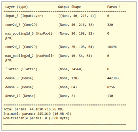
2.3 2D convolutional neural network
2-D CNN was created with the purpose of processing two-dimensional input, such as pictures. A 2-D CNN convolves these portions of the input by sliding filters across both height and width to return feature maps that emphasize relevant spatial features, such as Saad cropping, shapes, edges, and textures. In order to increase the network's computational efficiency while preserving as much information as feasible, pooling layers shrink these feature maps in the following stage. Fully connected layers at the back classify images, detect objects, and segment them. 2D CNNs have been a backbone for many state-of-the-art computer vision systems on account of their skill to pick up hierarchical representation from visual data [11].
2.4 Long short-term memory
LSTM is a specially designed RNN architecture that enables information to be forecast or learned over very long sequences by solving traditional RNN issues, essentially the vanishing gradient problem. This is through the memory cells within LSTMs and gating mechanisms: the input gate, the output gate, and the forget gate. All these control inflow, outflow, and internal flow that passes in every cell. In this line, LSTMs may maintain and update their cell state through which they might capture long-term dependencies in sequential information [12]. Therefore, areas of application for LSTMs include time series prediction, natural language processing, speech recognition, and many more such related processes that need understanding of the context over a long sequence.
2.5 Auto encoder
A deep neural network called an autoencoder efficiently encodes and decodes data via unsupervised feature learning. First, the AE compresses the data into a lower dimension’s latent space and then restores the data by decompression. The first step would be to use this unsupervised deep learning approach to learn an auto encoder as a compressed representation of input data for the identification of heart disease. Next, use this representation to categories or identify abnormalities. At the output layer, neural networks known as auto-encoders attempt to reassemble their input [13].
2.6 Data sources
In this work, the publicly available 2016 PhysioNet Challenge [14] heart sound dataset is considered. 3,240 heart sound recordings, ranging in length from 5 seconds to more than 2 minutes, are included in the collection. Both healthy and ill people were among the varied persons who made these recordings, and they did so in a variety of settings outside of clinical settings. Table 1 shows the dataset description of PhysioNet Challenge 2016 dataset.
Table 1. Dataset description
|
Heart Sound Dataset |
Abnormal Samples |
Normal Samples |
|
Training-a |
292 |
117 |
|
Training-b |
104 |
386 |
|
Training-c |
24 |
7 |
|
Training-d |
28 |
27 |
|
Training-e |
183 |
1,958 |
|
Training-f |
34 |
80 |
|
Total |
665 |
2,575 |
|
Total (Synthetic Data) Using GAN |
2525 |
2575 |
The literature innovatively provides recent and very major advances in the detection of heart disease using ML, DL and Transfer learning techniques for heart sound and signal analysis.
Machine learning and deep learning algorithms for heart disease detection using noisy sound signals from cardiac audios and datasets from the PASCAL CHALLENGE employ spectrograms, MFCCs, synthetic noise, and feature ensembles to visualize signals and categorize heart states [15]. Both studies demonstrate accurate diagnosis of heart problems based on sound inputs.
Transfer learning with pre-trained convolutional neural networks in resource-constrained settings for automatic PCG acoustic classification is investigated, and models trained on both audio and image modalities are fine-tuned using traditional time-frequency representations as input features [16]. The YAMNet-based TL method classifies four different types of heart sound data from public databases with 99.83% accuracy, 99.59% sensitivity, and 99.90% specificity. A strategy for synthesizing realistic PCG and ECG signals using LSGAN and Cycle GAN architectures is presented [17], and pre-trained CNN models are used to classify normal and pathological heartbeats from phonocardiogram data [18]. According to the experimental findings, audio-based models perform well; the VGGish model has the highest rate of true positives and average validation accuracy.
Convolutional neural networks on spectrograms [19], mel-spectrograms, and scalograms, achieving 91.25% accuracy on the PhysioNet Computing in Cardiology Challenge 2016 dataset, compared to 81.48% in the previous study. Data augmentation strategies can enhance the generalization capabilities of deep learning models for sound categorization, improving medical diagnostics [20, 21]. This approach addresses issues with restricted and imbalanced datasets in cardiovascular health research, resulting in more accurate and reliable heart disease prediction models.
A method for creating synthetic data with balanced attributes, marking a significant advancement in generative modelling [22]. Data augmentation tactics and model fusion procedures are used to improve the performance and resilience of arrhythmia detection models [23]. Additionally, a different transform called the chaogram is proposed to convert heart sound signals into coloured images [24]. Heart sounds are classified using deep convolutional neural networks while the data is converted by transfer learning algorithms. Their model had an accuracy as high as 88.06%. The continuous wavelet transform is used to create transfer learning models that can recognize six types of phonocardiogram recordings. Combining an open database with one class of heart sound data, including pulmonary hypertension, improves robustness in noisy conditions [25]. The system was trained with background deformation techniques and tested against ten transfer learning networks.
The study [26] transformed cardiac sound waves into a pattern-based spectrogram using PhysioNet 2016 and PASCAL 2011 datasets. Transfer Learning models like ResNet, DenseNet, MobileNet, Xception, VGG16, and InceptionV3 were used to categorize cardiac sounds as normal or abnormal. DenseNet outperformed rival models.
A method for the automatic analysis of heart sounds to detect symptoms of left ventricular diastolic dysfunction is developed, using a deep convolutional GAN model-based data augmentation technique to augment an LVDD-HS database for model training [27]. These techniques were compared with other methods for the detection of LVDD. Narváez Pedro et al. suggested a GAN-based approach for the generation of synthetic cardiac sounds, where they try to get accurate representations of typical heart sounds by coupling GAN with EWT capabilities in signal processing and extraction of features.
Synthetic heart sounds are generated using mathematical models to create the S1 and S2 phases of the cardiac cycle; however, modelling of systolic and diastolic periods is poor and renders them unsuitable to train heart rate classification models [28, 29]. Even a simple time-frequency analysis shows relevant differences regarding real signals.
Recent research has focused extensively on utilizing various techniques for heart disease detection based on heart sound signals. Researcher utilizes MFCCs, and synthetic noise alongside feature ensemblers to accurately categorize heart states using noisy sound signals and datasets like PASCAL and Physionet. Research explore transfer learning with pre-trained CNNs for automatic phonocardiogram (PCG) classification, achieving high accuracies using time-frequency representations. Other advancements include the synthesis of realistic PCG and ECG signals through GAN architectures as well as data augmentation strategies to enhance model generalization in cardiovascular health diagnostics.
Together, these findings demonstrate important advancements in the use of synthetic data methods and deep learning models to increase the precision and resilience of heart disease diagnosis and prediction systems. Literature work focuses on data augmentation techniques used to generate synthetic heart sound data that mostly be used to generate normal heart sounds.
The suggested study's primary features are:
The proposed architecture aims to expand a GAN-based model to address class imbalance in heart sound datasets and subsequently apply feature extraction, proposed Dl and transfer learning techniques for heart sound classification. This GAN framework is trained adversarial to generate balanced heart sound data, mitigating class imbalance issues. Following data generation, Feature extraction techniques such as MFCC, chroma, and spectral contrast are applied to capture discriminative characteristics from both real and synthetic heart sound data. The extracted features are then utilized as input to ML models such as KNN, KNN+ Feature Fusion, KNN+ feature Fusion+ hypermeters, DL classification models such as 1D CNN,2D CNN, LSTM, hybrid CNN-autoencoder and Transfer Learning Models such as VGG16, MobileNet for accurate classification of heart sounds across different cardiac conditions. By fine-tuning these pre-trained models on the balanced heart sounds dataset, the models can adapt their learned representations to better capture the unique characteristics of heart sounds, thereby enhancing classification performance. Figure 2 depicts the suggested architecture, and the processes are covered in the section following.
4.1 Load dataset and preprocessing
This step involves acquiring a dataset containing PhysioNet heart signal recordings. The dataset is labelled with different classes of heart signals, such as normal and abnormal then Label Encoding is performed. Label encoding is a ML approach that converts category input into numerical values. During this process, each unique category or label in the categorical variable is allocated a distinct integer value. In our work the labels are abnormal and normal heart sound signals which are converted into 0 and 1 using label encoding. Resampling a signal involves changing its sampling rate, which is done to prepare data for analysis at a different frequency.
4.2 Proposed GAN model
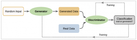
A Step GAN is employed for data balancing by generating synthetic heart sound signals to augment underrepresented classes. In order to improve the dataset's balance and support the development of reliable models for heart sound classification, the Generator generates new heart sound signals while the Discriminator separates actual from synthetic signals. The GAN Model's operation [30] is shown in Figure 3.
Figure 2. Proposed system architecture
Figure 3. Working of GAN model
Below are the steps to generate synthetic data using GAN model:
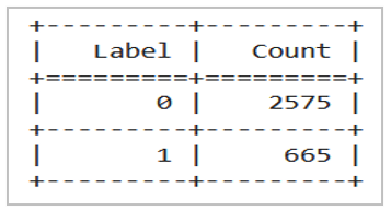
i) Calculate Label Count (Data Imbalance): Dataset analysed to determine the number of .WAV files per class (label). Calculated the count of samples for each class to identify any data imbalance issues.
ii) Get Label with Less Number of Class: Identify the class (label) with the least number of .WAV files. This is the class that needs generation. Figure 4 shows labels and its count.
Figure 4. Label count
iii) Apply Inception Model to Generate .WAV File.
Using an Inception-based model for .WAV file generation entails creating a GAN architecture that uses an Inception-like structure as the generator. Design the generator network architecture, which will have an Inception-like topology. Inception models often use numerous parallel convolutional routes with varying filter sizes.
Random noise and latent spatial representation are accepted by the generator. Create a discriminator network design that can differentiate between created and real data. WAV files.
A CNN architecture created for audio classification serves as the discriminator. Train the GAN model with a real-world dataset.WAV files. During training, the generator attempts to provide realistic results.WAV files that can deceive the discriminator while it learns to tell the difference between real and created.WAV files.
Generator: The generator is designed to generate data with a specific shape. It starts with a sequential model and adds layers sequentially. The first is a dense layer of 12*1000 units with a LeakyReLU activation function, no bias. Batch normalization is applied just after this layer. Further reshaping of the data in this example is into a 3D shape: (1000, 12). The next step will be to add three convolutional 1D transpose layers, gradually reducing the number of filters from 256 to 128, then to 64, and finally to 32. Batch Normalisation and LeakyReLU activation come after each convolutional layer. The last convolutional layer uses tanh as the activation. Assertions are included to ensure that the output shapes are per dimension. The generator model is then returned. Figure 5 depicts generator model architecture diagram.
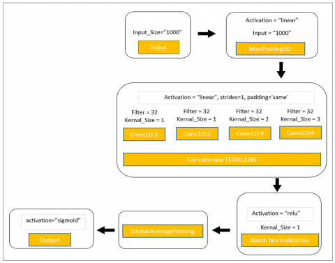
Discriminator: The discriminator network is crucial in adversarial learning, particularly in models like GANs. Its principal function is to identify between genuine and fabricated samples created by the generator network. The ` discriminator` function constructs the complete discriminator network. Building it starts with an input layer of a given, predetermined shape. In order to minimize the spatial dimensions of the resulting tensor, this entails applying numerous inception modules sequentially with optional residual connections based on the truthy or falsy value of the `use_residual` parameter. Following these inception modules, global average pooling is applied. Lastly, a dense layer with a sigmoid activation function is used for binary classification, which determines if a transaction is genuine or fraudulent. Majorly, the discriminator network's role is to efficiently learn distinguishing characteristics from the input data and provide relevant knowledge regarding the same to a generator network in adversarial training. Figure 6 depicts desciminator model architecture diagram.
Figure 5. Generator model architecture diagram
Figure 6. Discriminator model architecture diagram
The model uses independent modules, inception modules and residual connections, to enhance its learning capacity without losing its stability during training. Filter sizes in inception module are described in Table 2 while Summary table with filter sizes and parallel path of generator and descriminator are shown in Table 3.
Table 2. Filter sizes in inception module (with parallel path)
|
Path |
Filter Size |
Kernel Size |
|
Conv1D Path 1 |
32 |
kernel_size // 1 = 40 (default) |
|
Conv1D Path 2 |
32 |
kernel_size // 2 = 20 |
|
Conv1D Path 3 |
32 |
kernel_size // 4 = 10 |
|
MaxPool + Conv1D Path |
32 |
1 (Conv1D after MaxPool) |
Table 3. Summary table with filter sizes and parallel path
|
Component |
Parallel Paths (Count) |
Filter Sizes |
|
Generator |
No |
Conv1DTranspose: [128, 64, 32, 12] |
|
Discriminator |
Yes (4 Parallel Branches) |
Conv1D (40, 20, 10) + Conv1D (1) |
4.3 Feature extraction
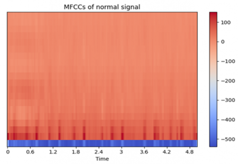
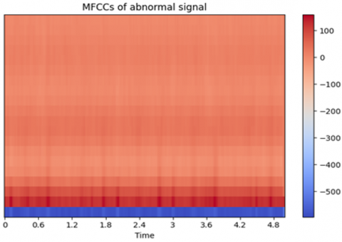
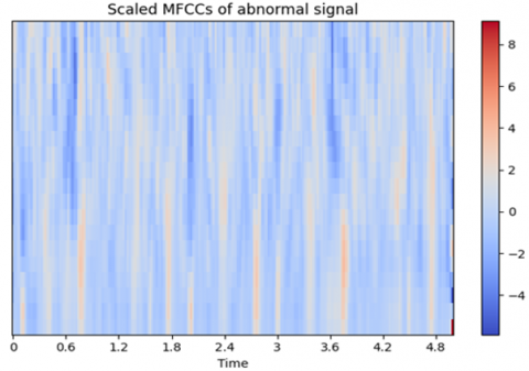
MFCC, Fast Fourier Transform, Wavelet, and Feature Fusion Technique are just a few of the feature extraction methods that have been used thus far on the heart signal data. By using the MFCC, chroma, and spectral contrast approaches to extract these qualities from audio, crucial information about the audio's spectral shape, pitch content, and timbral aspects can be obtained. These characteristics support the ability of deep learning and machine learning classifiers to identify patterns and provide predictions using the information gathered from the audio signals. MFCC, Chroma, STFT, and Spectral Contrast were selected due to their proven effectiveness in capturing the essential characteristics of audio signals relevant to PCG classification. MFCCs are well-suited for modeling the timbral texture of sound and are widely used in audio recognition tasks for their ability to mimic human auditory perception. Chroma features capture harmonic and tonal content, which helps in identifying pitch-related anomalies in heart sounds. Spectral Contrast emphasizes the difference between spectral peaks and valleys, aiding in the detection of subtle variations in signal energy. STFT provides a time-frequency representation that preserves both spectral and temporal information, essential for analyzing dynamic patterns in heart sounds. Compared to wavelet transforms, which are effective but more computationally intensive and complex to tune, the chosen features offer a balanced trade-off between interpretability, computational efficiency, and classification performance. MFCC of normal and abnormal signal shown in Figures 7(a) and (b) and Scaled MFCC of normal and abnormal signal given in Figures 8(a) and (b).
(a)
(b)
Figure 7. (a) MFCC of normal signal (b) MFCC of abnormal signal
(a)
(b)
Figure 8. (a) Scaled MFCC of normal signal (b) Scaled MFCC of abnormal signal
4.4 Feature reduction
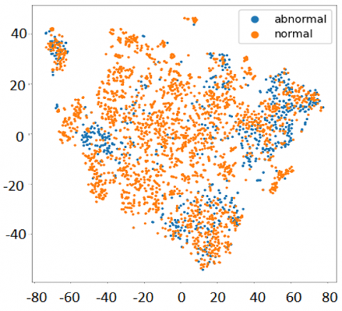
T-SNE,also known as t-distributed stochastic neighbor embedding. It is primarily used for reducing the dimensions of the data so that it can be visualized. But unlike PCA, which is mainly used for feature reduction, it can also, to some extent, provide feature selection by mapping high-dimensional space data onto lower-dimensional space while preserving its integrity. Feature Distribution is depicted in Figure 9.
Figure 9. Features distribution
4.5 Algorithms
K-nearest neighbors (KNN) used for heart sound classification by first extracting relevant features from heart sound recordings, such as frequency-domain characteristics or time-domain parameters. These features are utilised to represent each instance of a heart sound in a multidimensional feature space. Throughout the training phase, KNN retains these feature vectors alongside their respective class labels. Following steps performed for classification with KNN: KNN (MFCC Features), KNN (MFCC Features with TSNE Feature Reduction, KNN (MFCC with Spectral Amplitude / FFT Features), KNN (Wavelet Based Features), KNN (Feature Fusion Technique), KNN (Hyper Parameters Tuning).
4.5.1 KNN with feature fusion+ hyper parameters tuning
The fusion of features in K-nearest Neighbors involves the combination of several feature sets in the model for enhanced performance. It provides better representation as it would be more prosperous and more comprehensive with information about the data. This is done by concatenating in one set the abundances from different feature sets, scaling accordingly, and optionally applying dimensionality reduction methods. These feature sets are then tuned with hyperparameters associated with the optimization of some main parameters of the KNN algorithm, that is, the number of neighbors. KNN has a hyperparameter, k, which represents the number of neighbors to consider. Use techniques random search to search for the optimal value of k. Evaluate the performance of KNN with different values of k using cross-validation. Select the value of k that yields the best performance on validation set. Combining feature fusion and optimizing KNN hyperparameters is done random searches with cross-validation because of its capability to leverage several data aspects while determining the best configuration for a KNN model.
4.5.2 Proposed hybrid CNN + autoencoder
It combines CNNs for feature extraction and autoencoders for unsupervised learning. Use a CNN to process raw audio data or spectrogram images and extract meaningful features. Connect the output of the CNN to an autoencoder architecture to learn a compressed representation of the features.
A hybrid model combining an autoencoder with a 1D convolutional network for a binary classification problem. First, an efficient format of the input data was learnt by successively applying an autoencoder in an unsupervised pre-training way. The learnt features are then applied to the classification issue by reshaping this learnt representation and feeding it into a 1D convolutional network.
In this model, there will be a Dropout layer wherein, during training, a portion of the input units will be zeroed at every update. Likely, the latter prevents overfitting so that the model does not become too biased toward particular features from the input.
Output Layer: The predicted probabilities for the binary classification challenge are obtained using a fully associated Dense layer with softmax activation. CNN-autoencoder model architecture shown in Figure 10.
Figure 10. CNN-autoencoder model architecture
4.5.3 Transfer learning algorithms:
Pre-trained models VGG16 and MobileNet are applied on both balanced and unbalanced heart sound datasets.
VGG16:
A deep convolutional neural network model called VGG16 was created specifically for image classification. The network consists of 16 layers of artificial neurones, each of which improves prediction accuracy by sequentially interpreting image data.
VGG 16 Network Architecture: The network consists of five convolutional blocks followed by a classification block. Architecture Diagram of VGG16 shown in Figure 11.
Each convolutional block contains:
Step 1: Uses Conv1D layers for 1-dimensional convolution suitable for audio data.
Step 2: Applies ReLU activation for non-linearity.
Step 3: Uses max pooling for downsampling.
Step 4: Includes dropout for regularization (preventing overfitting).
The classification block contains:
Step 1: Flattens the convolutional output into a 1D vector.
Step 2: Uses fully-connected layers (Dense) with ReLU activation for learning higher-level features.
Step 3: Outputs through a final dense layer with:
MobileNet:
Google developed MobileNet, a convolutional neural network (CNN) architecture, especially for embedded and mobile vision applications. The goal is to develop efficient, lightweight models that can be utilised on low-resource devices. To reduce the amount of parameters and computational complexity without sacrificing performance, the architecture places a high priority on the use of depthwise separable convolutions.
MobileNet Network Architecture:
Step 1: Input Layer: input_layer: This defines the input layer that receives the pre-processed WAV file data.
Step 2: Convolutional Blocks (1-5):
Each block follows a similar pattern:
DepthwiseConv1D: Applies a depthwise separable convolution to extract features efficiently.
Conv1D: Applies a pointwise convolution to increase the number of filters.
MaxPooling1D: Preserves significant properties while reducing the data's dimensionality.
Dropout: Randomly drops a percentage of activations to prevent overfitting.
Classification Block:
Flatten: Transforms the convolutional blocks' multi-dimensional output into a single dimension so that it may be fed into fully connected layers.
Dense layers (dense1-dense3): These layers, which are fully integrated, discover intricate connections between the heart sound classes and the retrieved attributes.
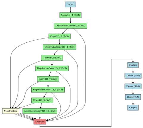
Output: The final output layer with the number of units depending on the output_number and activation function based on the problem_type. (Softmax for classification, linear for regression).Figure 12 depicts the mobilenet architecture diagram.
Figure 11. VGG 16 architecture diagram
Figure 12. MobileNet architecture diagram
5.1 Experimental setup
To run the models, setup typically involves utilizing Google Colab's resource and Python as technology. A practical and robust cloud-based environment for carrying out machine learning and deep learning experiments is provided by Google Colab. With Python 3.10 as the programming language of choice. By selecting the appropriate runtime type, and access GPU acceleration, which significantly speeds up the training of DL and transfer learning models compared to running on CPUs alone. Additionally, Colab provides ample RAM, with around 12 GB available in the standard runtime environment and up to 25 GB in the high-RAM runtime environment and GPU 5GB.
5.2 Performance parameters
The most common measures to calculate the effectiveness of a classifier include accuracy, precision, recall, and F1-score.
Precision $=\frac{\mathrm{TP}}{\mathrm{TP}+\mathrm{FP}}$ (2)
Accuracy $=\frac{\mathrm{TP}+\mathrm{TN}}{\mathrm{TP}+\mathrm{TN}+\mathrm{FP}+\mathrm{FN}}$ (3)
Recall / Sensitivity $=\frac{\mathrm{TP}}{\mathrm{TP}+\mathrm{FN}}$ (4)
$F 1-$ Score $=2 * \frac{(\text { Precision }+ \text { Recall })}{(\text { Precision } * \text { Recall })}$ (5)
Accuracy and Loss curve: While the loss curve displays the trend of the loss function—basically a measure of the discrepancy between predictions and actual labels—the accuracy curve illustrates the model's learning over time.
5.3 Results
Macro-average is used to aggregate metrics such as precision, recall, or the F1 score over many classes of a classification task. The macro average computes this metric independently for each class and thereafter takes the average. All classes are given equal weight in its computation, totally disregarding class imbalance, hence providing an equal contribution from each class to the total metric. Macro-averaging is preferred for imbalanced datasets because it treats all classes equally, giving equal importance to minority and majority classes. In contrast, weighted-averaging gives more weight to frequent classes, which can hide poor performance on under-represented ones.
In the proposed work, a GAN-based Inception model is used to generate balanced heart sound data to overcome the class imbalance issue in the PhysioNet dataset. Considering all the training folders for the PhysioNet dataset, 2575 samples represent normal heart sound signals, and 665 samples represent abnormal heart sound signals. To balance the representation of both classes, an Inception-based GAN was used to increase the samples of abnormal heart sounds. Table 4 shows Hyperparameters used in Inception based GAN model. In a generator, gradients are crucial for learning. The standard ReLU activation can lead to the dying ReLU problem, where neurons output zero for all inputs and stop learning. LeakyReLU, on the other hand, allows a small, non-zero gradient when the unit is not active (typically 0.01 * x), helping the generator keep learning even when activations are negative.
In parameters tuning the batch size (32) is selected to balance training speed, memory efficiency, and gradient stability.
The generator network generates 1,910 fresh samples of aberrant heart sounds once the discriminator and generator networks have been trained for 800 epochs. Then, the generated abnormal heart sound signals will be combined with original abnormal heart sound signals, which will provide a balanced representation of both normal and abnormal heart sounds. Out of all the recordings, 80% of the samples pass training, and 20% pass testing. Both balanced and unbalanced heart sounds are used for classification. Analysis was done on existing models for predicting heart failure based on heart sound data.
Table 4. Hypermarameters of inception based GAN model
|
Parameters |
Generator Parameter Values |
Discriminator Parameter Values |
|
Loss Function |
Binary-Cross Entropy |
Mean Absolute Error (MAE) |
|
Activation Function |
LeakyRelu, Tanh |
Relu, Sigmoid |
|
Batch size |
32 |
32 |
|
Kernel size |
5 |
1,2,3 |
|
Filter size |
16,32,64 |
32,128 |
|
Learning Rate |
0.0004 |
0.001 |
|
Number of Epoch |
800 |
|
The generator and discriminator network are trained for 800 epochs, after which the Generator Network produces 1,910 new samples of abnormal heart sounds. Figure 13 shows Sample generated of synthetic heart sound signal using GAN Model. Then, the generated abnormal heart sound signals will be combined with original abnormal heart sound signals, which will provide a balanced representation of both normal and abnormal heart sounds. From total recordings 80% samples are passed for training and 20% passed for testing. Classification of heart sounds is done on both balanced and unbalance heart sounds. Existing models for Heart Failure Prediction using Heart Sound data were analysed. Various techniques such as feature extraction, feature selection, feature fusion, and hyperparameter tuning were applied to the KNN algorithm.
It shows that KNN ((Feature Fusion+ Hyper Parameters Tuning) outperforms better than KNN(MFCC), KNN (MFCC Features with TSNE Feature Reduction), KNN (MFCC with Spectral Amplitude / FFT Features), KNN (Feature Fusion Technique). Deep learning algorithms including 1D-CNN, 2D-CNN, LSTM and proposed hybrid CNN+Auto Encoder, and transfer learning algorithms such as MobileNet and VGG16 were also utilised.
The results shows that the Proposed Hybrid CNN + Auto Encoder achieves an accuracy of 97%, whereas MobileNet achieves 93% accuracy and VGG16 achieves 91% accuracy.
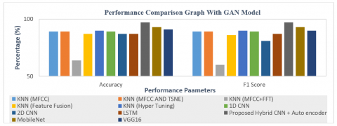
The proposed hybrid CNN + Autoencoder model demonstrates superior performance compared to existing models, specifically 1D-CNN, 2D-CNN, and LSTM. Performance is calculated on different algorithms using various performance measures such as accuracy, precision, recall, and F1-score. Table 5 shows the comparison with and without GAN Model. It shows that F1 score is comparatively good in GAN model that balances both precision and recall, making it useful in dealing with imbalanced datasets.
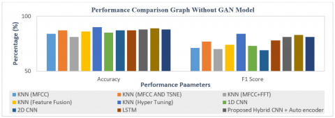
Figure 14 shows the accuracy and macro F1-score graph of different algorithms without GAN Model. Figure 15 shows performance comparison with GAN model. It has been shown that in addition to accuracy, the macro F1 score also yields favourable outcomes for all machine learning, deep learning, and transfer learning algorithms. The F1 score is a measure that combines precision and memory by taking their harmonic mean. Maximising the F1 score means maximising both precision and recall at the same time. Figure 16. gives the F1 score comparison of algorithms with and without GAN model. It is observed that F1 score is increased by minimum 5% to a maximum 15% using GAN model. F1-score with GAN model getting Improved performance with KNN Hyper parameter tuning, and Proposed Autoencoder + CNN, Fine-tune MobileNet and VGG16 algorithm.
Table 5. Comparison of different classifiers performance measures with and without GAN model
|
Algorithms |
Accuracy |
Precision |
Recall |
F1-Score |
|
|
Without GAN Model (Macro Avg in %) |
|||
|
KNN (MFCC Features) |
84 |
78 |
68 |
71 |
|
KNN (MFCC Features with TSNE Feature Reduction) |
87 |
80 |
75 |
77 |
|
KNN (MFCC with Spectral Amplitude / FFT Features) |
81 |
71 |
69 |
70 |
|
KNN (Proposed Feature Fusion Technique) |
86 |
75 |
74 |
74 |
|
KNN (Feature Fusion+ Hyper Parameters Tuning) |
90 |
86 |
82 |
84 |
|
1D CNN |
85 |
81 |
70 |
73 |
|
2D CNN |
87 |
85 |
65 |
69 |
|
LSTM |
87 |
81 |
75 |
78 |
|
Proposed Hybrid CNN + Auto Encoder |
88 |
84 |
79 |
81 |
|
MobileNet |
89 |
86 |
81 |
83 |
|
VGG16 |
88 |
81 |
80 |
81 |
|
|
With GAN Model (Macro Avg in %) |
|||
|
KNN (MFCC Features) |
89 |
91 |
89 |
89 |
|
KNN (MFCC Features with TSNE Feature Reduction) |
89 |
91 |
89 |
89 |
|
KNN (MFCC with Spectral Amplitude / FFT Features) |
64 |
79 |
66 |
60 |
|
KNN (Proposed Feature Fusion Technique) |
87 |
88 |
86 |
86 |
|
KNN (Hyper Parameters Tuning) |
90 |
90 |
89 |
90 |
|
1D CNN |
89 |
89 |
89 |
89 |
|
2D CNN |
87 |
85 |
84 |
81 |
|
LSTM |
87 |
87 |
87 |
87 |
|
Proposed Hybrid CNN + Auto encoder |
97 |
96 |
96 |
96 |
|
MobileNet |
93 |
93 |
93 |
93 |
|
VGG16 |
91 |
91 |
90 |
90 |
Figure 13. Original heart sound signal and generated heart sound signal
Figure 14. Performance comparison graph without GAN model
Figure 15. Performance comparison graph with GAN model
Figure 16. F1 score comparison graph of algorithms with and without GAN model
(a)
(b)
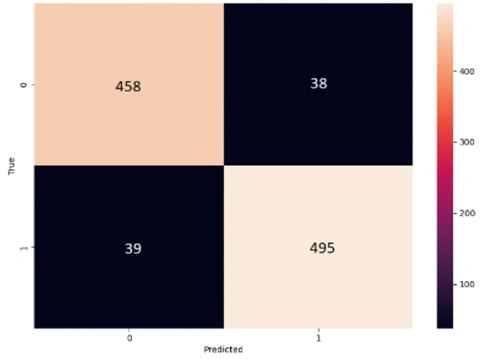
Figure 17. Confusion matrix a) MobileNet b) Hybrid CNN + Autoencoder
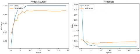
Figure 18. Hybrid CNN + Autoencoder accuracy and loss curve
The confusion matrix of the MobileNet and Proposed Hybrid CNN+Autoencoder model is depicted in Figure 17 and Accuracy and Loss Curve of the MobileNet and Proposed Hybrid CNN+Autoencoder is depicted in Figure 18. The classification results show better improvement using these algorithms. Total 1030 recordings are considered for testing purpose after data balancing. The MobileNet accurately recognized 458 out of 496 abnormal samples and 495 out of 534 normal samples. The Hybrid CNN+Autoencoder accurately recognized 470 out of 496 abnormal samples and 524 out of 534 normal samples. The misclassification of 38 abnormal samples by MobileNet is primarily due to imperfections and distribution gaps in the GAN-generated synthetic data. Despite appearing realistic, synthetic abnormalities might introduce subtle inconsistencies and feature overlaps, challenging MobileNet’s limited feature extraction capacity. Consequently, these factors significantly impact the model’s ability to accurately distinguish abnormal classes. Figure 19 shows the Mobilenet accuracy and loss curve.
Figure 19. Mobilenet accuracy and loss curve
Result Findings
This paper proposes an approach to tackle the problem of the imbalanced dataset in the classification of CHF using an inception-based GAN model. Since collecting many samples of a specific type of abnormality is strongly felt challenging, a GAN-based model was created that generates abnormal heart sounds. An Inception-based GAN model is used here because of the powerful feature extraction capabilities of the Inception architecture, leading to higher quality and more realistic synthetic heart sound signals compared to traditional GANs. Further, techniques such as feature extraction using MFCCs, chroma, and spectral contrast used on both unbalanced and balanced heart sound data to extract discriminative features.
Moreover, the proposed Hybrid CNN + Autoencoder model showed the best performance in all the main evaluation metrics, as it could reach 98% accuracy and 97% F1 score with the rank of GAN-augmented dataset. Also, fine-tuned transfer learning models like MobileNet and VGG16 gave the extra kick in performance. This integrated methodology both increased accuracy and increased macro-averaged recall and F1-score up to 5% to 15% when detecting both normal and abnormal heart sounds. It is shown at an overall level, however, that performing synthetic data generation in conjunction with deep feature fusion and hybrid deep learning architectures represents a viable framework to further automated CHF detection. These findings pose support for the use of GANs and autoencoder driven approach to improve the existing Cardiovascular diagnostic using intelligent, data driven solutions. Attention Mechanisms can be incorporated into the Autoencoder Framework for the feature learning as a further work. Also, real time deployment on wearable device enables it to support continuous monitoring of heart sound which facilitates early detection of CHF.
[1] Di Cesare, M., Perel, P., Taylor, S., Kabudula, C., Bixby, H., Gaziano, T.A., McGhie, D.V., Mwangi, J., Pervan, B., Narula, J., Pineiro, D., Pinto, F.J. (2024). The heart of the world. Global Heart, 19(1): 11. https://doi.org/10.5334/gh.1288
[2] Etoom, Y., Ratnapalan, S. (2014). Evaluation of children with heart murmurs. Clinical Pediatrics, 53(2): 111-117. https://doi.org/10.1177/0009922813488653
[3] Bizopoulos, P., Koutsouris, D. (2018). Deep learning in cardiology. IEEE Reviews in Biomedical Engineering, 12: 168-193. https://doi.org/10.1109/RBME.2018.2885714
[4] Gawande, N., Goyal, D. (2023). Empirical review on heart failure detection techniques using heart sound. AIP Conference Proceedings, 2782(1): 020037. https://doi.org/10.1063/5.0154522
[5] Ali, L., Rahman, A., Khan, A., Zhou, M., Javeed, A., Khan, J.A. (2019). An automated diagnostic system for heart disease prediction based on χ2 statistical model and optimally configured deep neural network. IEEE Access, 7: 34938-34945. https://doi.org/10.1109/ACCESS.2019.2904800
[6] Sarra, R.R., Dinar, A.M., Mohammed, M.A., Ghani, M.K.A., Albahar, M.A. (2022). A robust framework for data generative and heart disease prediction based on efficient deep learning models. Diagnostics, 12(12): 2899. https://doi.org/10.3390/diagnostics12122899
[7] Gawande, N., Goyal, D., Sankhla, K. (2024). Improved deep learning and feature fusion techniques for chronic heart failure. International Journal of Intelligent Systems and Applications in Engineering, 12(17s): 67-80.
[8] Abbas, S., Ojo, S., Al Hejaili, A., Sampedro, G.A., Almadhor, A., Zaidi, M.M., Kryvinska, N. (2024). Artificial intelligence framework for heart disease classification from audio signals. Scientific Reports, 14(1): 3123. https://doi.org/10.1038/s41598-024-53778-7
[9] Jabbar, M.A., Deekshatulu, B.L., Chandra, P. (2013). Classification of heart disease using K-nearest neighbor and genetic algorithm. Procedia Technology, 10: 85-94. https://doi.org/10.1016/j.protcy.2013.12.340
[10] Honi, D.G., Szathmary, L. (2024). A one-dimensional convolutional neural network-based deep learning approach for predicting cardiovascular diseases. Informatics in Medicine Unlocked, 49: 101535. https://doi.org/10.1016/j.imu.2024.101535
[11] Arooj, S., Rehman, S.U., Imran, A., Almuhaimeed, A., Alzahrani, A.K., Alzahrani, A. (2022). A deep convolutional neural network for the early detection of heart disease. Biomedicines, 10(11): 2796. https://doi.org/10.3390/biomedicines10112796
[12] Sudha, V.K., Kumar, D. (2023). Hybrid CNN and LSTM network for heart disease prediction. SN Computer Science, 4(2): 172. https://doi.org/10.1007/s42979-022-01598-9
[13] Khozeimeh, F., Sharifrazi, D., Izadi, N.H., Joloudari, J.H., Shoeibi, A., Alizadehsani, R., Gorriz, J.M., Hussain, S., Sani, Z.A., Moosaei, H., Khosravi, A., Nahavandi, S., Islam, S.M.S. (2021). Combining a convolutional neural network with autoencoders to predict the survival chance of COVID-19 patients. Scientific Reports, 11(1): 15343. https://doi.org/10.1038/s41598-021-93854-1
[14] Liu, C., Springer, D., Li, Q., et al. (2016). An open access database for the evaluation of heart sound algorithms. Physiological Measurement, 37(12): 2181. https://doi.org/10.1088/0967-3334/37/12/2181
[15] Rashwan, A.R., El Fangary, L., Azzam, S.M. (2023). Predicting heart disease using modified GoogLeNet convolutional neural network architecture based on the heart sound. Information Sciences Letters, 12(11): 2837-2858. https://doi.org/10.18576/isl/121101
[16] Maity, A., Pathak, A., Saha, G. (2023). Transfer learning based heart valve disease classification from Phonocardiogram signal. Biomedical Signal Processing and Control, 85: 104805. https://doi.org/10.1016/j.bspc.2023.104805
[17] Rayavarapu, S.M., Prasanthi, T.S., Kumar, G.S., Rao, G.S., Prashanti, G. (2023). A generative model for deep fake augmentation of phonocardiogram and electrocardiogram signals using LSGAN and Cycle GAN. Informatyka, Automatyka, Pomiary w Gospodarce i Ochronie Środowiska, 13(4): 34-38. http://doi.org/10.35784/iapgos.3783
[18] Alrabie, S., Barnawi, A. (2023). Evaluation of pre-trained CNN models for cardiovascular disease classification: A benchmark study. Information Sciences Letters, 12(7): 3317-3338. https://doi.org/10.18576/isl/120755
[19] Marocchi, M., Abbott, L., Rong, Y., Nordholm, S., Dwivedi, G. (2023). Abnormal heart sound classification and model interpretability: A transfer Learning Approach with Deep Learning. Journal of Vascular Diseases, 2(4): 438-459. https://doi.org/10.3390/jvd2040034
[20] Abayomi-Alli, O.O., Damaševičius, R., Qazi, A., Adedoyin-Olowe, M., Misra, S. (2022). Data augmentation and deep learning methods in sound classification: A systematic review. Electronics, 11(22): 3795. https://doi.org/10.3390/electronics11223795
[21] Susic D, Gradisek A, Gams, M. (2024). PCGmix: A data-augmentation method for heart-sound classification. IEEE Journal of Biomedical and Health Informatics. 28(11): 6874-6885. https://doi.org/10.1109/JBHI.2024.3458430
[22] Doubinsky, P., Audebert, N., Crucianu, M., Le Borgne, H. (2022). Multi-attribute balanced sampling for disentangled GAN controls. Pattern Recognition Letters, 162: 56-62. https://doi.org/10.1016/j.patrec.2022.08.012
[23] Ma, S., Cui, J., Xiao, W., Liu, L. (2022). Deep learning-based data augmentation and model fusion for automatic arrhythmia identification and classification algorithms. Computational Intelligence and Neuroscience, 2022(1): 1577778. https://doi.org/10.1155/2022/1577778
[24] Harimi, A., Majd, Y., Gharahbagh, A.A., Hajihashemi, V., Esmaileyan, Z., Machado, J.J., Tavares, J.M.R. (2022). Classification of heart sounds using chaogram transform and deep convolutional neural network transfer learning. Sensors, 22(24): 9569. https://doi.org/10.3390/s22249569
[25] Wang, M., Guo, B., Hu, Y., Zhao, Z., Liu, C., Tang, H. (2022). Transfer learning models for detecting six categories of phonocardiogram recordings. Journal of Cardiovascular Development and Disease, 9(3): 86. https://doi.org/10.3390/jcdd9030086
[26] Arora, V., Verma, K., Leekha, R.S., Lee, K., Gupta, T., Bhatia, K. (2021). Transfer learning model to indicate heart health status using phonocardiogram. Computers, Materials & Continua, 69(3): 2899-2917. https://doi.org/10.32604/cmc.2021.019178
[27] Yang, Y., Guo, X.M., Wang, H., Zheng, Y.N. (2021). Deep learning-based heart sound analysis for left ventricular diastolic dysfunction diagnosis. Diagnostics, 11(12): 2349. https://doi.org/10.3390/diagnostics11122349
[28] Narváez, P., Percybrooks, W.S. (2020). Synthesis of normal heart sounds using generative adversarial networks and empirical wavelet transform. Applied Sciences, 10(19): 7003. https://doi.org/10.3390/app10197003
[29] Karar, M.E., El-Brawany, M. (2016). Embedded heart sounds and murmurs generator based on discrete wavelet transform. In 2016 Fourth International Japan-Egypt Conference on Electronics, Communications and Computers (JEC-ECC), Cairo, Egypt, pp. 34-37. https://doi.org/10.1109/JEC-ECC.2016.7518962
[30] Abedi, M., Hempel, L., Sadeghi, S., Kirsten, T. (2022). GAN-based approaches for generating structured data in the medical domain. Applied Sciences, 12(14): 7075. https://doi.org/10.3390/app12147075