Jefri Junifer Pangaribuan*![]() | Justin Thames
| Justin Thames![]() | Romindo
| Romindo![]() | Okky Putra Barus
| Okky Putra Barus![]()
© 2024 The authors. This article is published by IIETA and is licensed under the CC BY 4.0 license (http://creativecommons.org/licenses/by/4.0/).
OPEN ACCESS
Nuts are an important product in the agricultural and food industry throughout the world where they contain vegetable protein, fibre and other important nutrients for the human diet. Each type of nut has its characteristics. In addition, manually classifying and sorting the nut seeds is very difficult to do. Therefore, it is very important to classify and identify the type of dry nut. Methods that can be used to classify types of nuts are the Support Vector Machine (SVM) method and Linear Discriminant Analysis (LDA). There are seven types of dry nuts with seven different levels of accuracy based on calculations per class using the SVM and LDA methods. The results of the accuracy of the SVM method are Barbunya at 98%, Bombay at 100%, Cali at 98%, Dermason at 96%, Horoz at 99%, Seker at 98%, Sira at 95% while the results of the accuracy of the LDA method are Barbunya at 98%, Bombay at 100%, Cali at 98%, Dermason at 95%, Horoz at 98%, Seker at 98%, Sira at 93%.
support vector machine, linear discriminant analysis, nut, classification, accuracy
Nuts are an important product in the agricultural and food industry throughout the world where they contain vegetable protein, fibre and other important nutrients for the human diet. Each type of nut has its characteristics, so it is very important to identify and classify the type of nut. Accurate classification is crucial for minimizing post-harvest damage, improving processing efficiency, and ensuring high-quality products for commercialization. By selecting and classifying peanut samples based on attributes like size and colour, producers can enhance the marketability and consumer acceptance of these products [1].
The main objective of this research is to compare the effectiveness of two machine learning algorithms, Support Vector Machine (SVM) and Linear Discriminant Analysis (LDA) in classifying various types of dry nuts. The motivation behind using these algorithms stems from their proven performance in other fields such as image processing [2, 3] medical diagnostics [4, 5] and financial forecasting [6, 7]. However, there has been limited exploration of their application in the agricultural domain, particularly for the classification of nuts. This research aims to address that gap by analyzing their accuracy and suitability for this specific task.
The SVM method is a classification method used to separate two data classes where the SVM method works by finding the largest margin between different data classes which is determined from the distance between the dividing line and the closest point of the two classes [8]. The SVM method aims to find the line separator that has the largest margin, so this makes it better at abstracting unknown data.
The way SVM works starts by visualizing each data point in dimensional space according to the features in the data. Then, a decision boundary or hyperplane will be formed which is used as a decision boundary that maximizes the distance or margin. The point that is closest between these classes is called the support vector. SVM projects data into dimensional space using a kernel function where this kernel function can help the SVM in creating an effective hyperplane. The way to determine the best hyperplane is to look for ideal lines that are divided into these two classes where the lines are not close to each other and are far from the two points. In other words, the line must be in the middle of both classes.
Several examples of the application of the SVM method which can be used in various application fields such as image classification [9], traffic casualties [10], genome classification [11], financial analysis [12], detecting cyberbullying on social media [13], identifying black-hole attacks to enhance Mobile Ad Hoc Network (MANET) security [14], and others. SVM has been previously used to predict the moisture content of Macadamia nut-in-shell [15].
LDA is a classification method used to separate two or more groups of data. LDA works by finding a linear combination of features that maximizes the differences between groups of data, making it easier to classify new data [16]. The way LDA works starts by calculating the mean, calculate the covariance matrix each class, calculate the in-class covariance matrix, and calculate the formation of linear discriminant functions.
Several examples of the application of the LDA method which can be used in various application fields such as facial recognition [17], disease detection [18], and others. LDA has also been employed in research to identify shelled and unshelled walnuts. LDA has been applied in research aimed at classifying shelled and unshelled walnuts [19].
Apart from the SVM and LDA method, there are several other methods that can be used to classify types of nuts, namely Decision Tree [20], Naïve Bayes [21], Artificial Neural Network (ANN) [22], and Logistic Regression [23]. Each of these methods needs to consider the type of data characteristics and the desired analysis objectives. The reason the researcher did not use this method was that there were shortcomings in each of these methods and they were not very suitable for this research, so the researcher decided to use the SVM and LDA methods in this research. This can be seen from the shortcomings of Naïve Bayes, namely that it lies in the predictors of the independent variables, which can slow down the classification performance [24], Random Forest also has a disadvantage, namely that it is difficult to interpret the influence of each feature in decision making [25], Logistic Regression also has a disadvantage, namely that it is sensitive to underfitting in datasets whose classes are not balanced, which will cause low accuracy values [26].
Table 1 is a summary of three previous and published research journals on topics related to classification results using SVM and LDA. Some of these journals can be used as comparisons and strengthen literature studies on the author's research topic.
Table 1. Comparison table of previous research
|
No. |
Writer’s Name |
Research Result |
|
1 |
Koklu and Ozkan [27] |
Based on the results obtained, the SVM method has the best level of accuracy compared to other methods, but the model can be further improved by using a hybrid of machine learning methods, deep learning and new algorithms. |
|
2 |
Ahmed et al. [28] |
Based on the results obtained, using a combination of PCA, LDA and KNN methods has the highest accuracy rate of 98% compared to SVM which only gets 97.4%. |
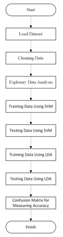
Figure 1. Flowchart of dry nut types classification stage
The detailed procedure for deriving classification results for different types of dry nuts from the dataset is depicted in Figure 1. This flowchart outlines each critical step involved, from initial data preparation to the application of specific classification algorithms.
2.1 Load dataset
First, launch the Jupyter Notebook application via the Command Prompt. Then, select the "New Notebook" option to create a new notebook. Download the dataset from the UCI Machine Learning Repository website beforehand. Once the dataset in .xlsx format is downloaded, upload it to the notebook by dragging and dropping the file.
2.2 Cleaning data
After the dataset is successfully uploaded, the next step was data cleaning. This step was essential to ensure that the dataset used for training and testing the models was accurate, consistent, and free from errors. Initially, we inspected the dataset for any missing values. The dataset was found to contain no missing values, so no imputation was necessary. Additionally, duplicate rows were checked, and no duplicates were found. However, we identified several outliers in the 'Perimeter' and 'MajorAxisLength' variables, which were disproportionately large compared to the majority of data points. These outliers were removed because they likely resulted from data entry errors or anomalies in the nut measurement process that could skew the model's performance.
Next, categorical variables were checked to ensure consistency in labelling. For example, the 'Class' column, which contained the nut type, was inspected for spelling errors or inconsistent capitalization. The data was also checked for any formatting issues, such as spaces or special characters, which were corrected to maintain consistency.
2.3 Exploratory data analysis
This stage has an important role in understanding the characteristics of the dataset and preparing the data for modeling. Before modeling, numerical variables such as 'Area', 'Perimeter', 'Eccentricity', and 'ShapeFactor1' were normalized using min-max scaling to ensure that all features were on a similar scale, which is crucial for algorithms like SVM and LDA that are sensitive to feature scaling. Normalization transforms the data into a range between 0 and 1, which helps improve the model’s convergence and performance.
For the categorical target variable ('Class'), which included seven nut types, label encoding was performed. This step was necessary because classification algorithms require numerical input, so each nut type was assigned a unique integer. This encoding process ensures that the models can correctly interpret the nut types as classes for prediction.
By following these detailed steps in cleaning and transforming the data, the dataset became well-prepared for the modeling process, ensuring more accurate and reliable results.
2.4 Class imbalance assessment
Upon analyzing the dataset, we observed that there was a class imbalance, with some nut types significantly outnumbering other.
2.5 Training data using SVM
At this stage, training data will be created to create a SVM model by studying existing patterns and relationships. The SVM model was trained using the Radial Basis Function (RBF) kernel, which is suitable for non-linear data classification. To optimize the model performance, we performed hyperparameter tuning using Grid Search, evaluating a range of values for the regularization parameter (C) and the kernel coefficient (gamma). The values of C were tested in the range of 0.1 to 10, while gamma was tested from 0.01 to 1. The best combination was selected based on cross-validation accuracy. Additionally, a stratified k-fold cross-validation with 10 folds was employed to ensure that each fold maintained the same proportion of classes as the entire dataset. This approach provided a more robust estimate of the model's performance.
2.6 Testing data using SVM
After training data is carried out, data testing will then be carried out. Testing data uses a SVM model that has been created on training data and will be used in testing data with data that has not been used.
2.7 Training data using LDA
At this stage, training data will be created to create a LDA model by studying existing patterns and relationships. Similar to the SVM model, LDA parameters were selected based on the characteristics of the dataset. The LDA model requires the computation of the mean vectors and the covariance matrices for each class, which was done using the training data. We ensured that the assumptions of LDA, including normally distributed data and equal covariance among classes, were validated through exploratory data analysis. Furthermore, the number of components to project the data onto was determined based on the number of classes minus one, which is a standard practice in LDA. This selection process enhances the model's ability to separate different classes effectively.
2.8 Testing data using LDA
After training data is carried out, data testing will then be carried out. Testing data uses a LDA model that has been created on training data and will be used in testing data with data that has not been used.
2.9 Confusion matrix
The final step is to measure the accuracy of the model that has been developed using confusion matrix.
In this research, the dataset was obtained from the UCI Machine Learning Repository website through this link, https://archive.ics.uci.edu/datasets. This dataset contains 17 variables listed in Table 2.
Table 2. Table of variables in the dataset [27]
|
No. |
Variable |
Description |
|
1 |
Area |
Describes the area of the nut which is calculated from the number of pixels within the bean's boundaries. |
|
2 |
Perimeter |
Describes the overall length of the edge of the nut. |
|
3 |
MajorAxisLength |
Describes the distance between the ends of the longest line on a nut. |
|
4 |
MinorAxisLength |
Describes the distance on the longest line perpendicular to the main axis. |
|
5 |
AspectRation |
Describes the comparison between MajorAxisLength and MinorAxisLength. |
|
6 |
Eccentricity |
Describes how oval the elliptical shape of a nut is. |
|
7 |
ConvexArea |
Describes the number of pixels in a convex polygon that contains the area of a nut. |
|
8 |
EquivDiameter |
Describes the diameter of a circle whose area is the same as the area of a nut. |
|
9 |
Extent |
Describes the comparison between the number of pixels in the bounding box and the actual area of the nut. |
|
10 |
Solidity |
Describes the calculation of the ratio of pixels on the nut's convex shell to the entire nut's total pixels. |
|
11 |
Roundness |
Describes the calculation of the roundness of a nut using the formula 4πA/P2. |
|
12 |
Compactness |
Describes the density of the shape of a nut using a formula |
|
13 |
ShapeFactor1 |
Describes various aspects of the shape or morphology of nuts. |
|
14 |
ShapeFactor2 |
Describes various aspects of the shape or morphology of nuts. |
|
15 |
ShapeFactor3 |
Describes various aspects of the shape or morphology of nuts. |
|
16 |
ShapeFactor4 |
Describes various aspects of the shape or morphology of nuts. |
|
17 |
Class |
The target variable includes seven types of dry nuts: Seker, Barbunya, Bombay, Cali, Dermosan, Horoz, and Sira. |
This dataset contains seven types of dry nut used in this research with data totalling 13, 611 considering the type, structure, shape and characteristics. This data will be used in developing a classification model that can differentiate between different types of dry nuts. Each type of dry nut is photographed using a high-resolution camera and will go through a segmentation process along with feature extraction including 12 dimensions and 4 types of shapes that describe the geometric characteristics of the dry nut. This data was provided to the UCI Machine Learning Repository on September 13, 2020 [29].
3.1 Load dataset
The dataset is provided in .xlsx format. After downloading, it can be uploaded to the notebook by dragging and dropping the file. Once the upload is complete, the dataset becomes accessible for further processing.
This dataset comprises 13,611 records and includes 17 columns or variables. These variables represent various attributes, as illustrated in Table 3.
Table 3. Dry bean dataset
|
Area |
Perimeter |
MajorAxisLength |
MinorAxisLength |
AspectRation |
Eccentricity |
ConvexArea |
EquivDiameter |
Extend |
|
28395 |
610.291 |
208.1781167 |
173.88747 |
1.197191424 |
0.54981219 |
28715 |
190.1410973 |
0.76392252 |
|
28734 |
638.018 |
200.5247957 |
182.7344194 |
1.097356461 |
0.41178525 |
29172 |
191.2727505 |
0.78396813 |
|
29380 |
624.11 |
212.8261299 |
175.9311426 |
1.209712656 |
0.56272732 |
29690 |
193.4109041 |
0.77811325 |
|
30008 |
645.884 |
210.557999 |
182.5165157 |
1.153638059 |
0.49861598 |
30724 |
195.4670618 |
0.78268127 |
|
30140 |
620.134 |
201.8478822 |
190.2792788 |
1.06079802 |
0.33367966 |
30417 |
195.896503 |
0.77309804 |
|
30279 |
634.927 |
212.5605564 |
181.5101816 |
1.171066849 |
0.52040066 |
30600 |
196.3477022 |
0.77568848 |
|
30477 |
670.033 |
211.0501553 |
184.0390501 |
1.146768336 |
0.48947789 |
30970 |
196.9886332 |
0.7624015 |
Table 3. Dry bean dataset (Continue)
|
Solidity |
Roundness |
Compactness |
ShapeFactor1 |
ShapeFactor2 |
ShapeFactor3 |
ShapeFactor4 |
Class |
|
0.988856 |
0.95802713 |
0.913357755 |
0.007331506 |
0.003147289 |
0.834222388 |
0.998723889 |
SEKKER |
|
0.9849856 |
0.88703364 |
0.953860842 |
0.006978659 |
0.003563624 |
0.909850506 |
0.998430331 |
SEKER |
|
0.98955877 |
0.94784947 |
0.908774239 |
0.007243912 |
0.003047733 |
0.825870617 |
0.999066137 |
SEKER |
|
0.97669574 |
0.90393637 |
0.928328835 |
0.007016729 |
0.003214562 |
0.861794425 |
0.994198849 |
SEKER |
|
0.99089325 |
0.98487707 |
0.970515523 |
0.00669701 |
0.003664972 |
0.941900381 |
0.999166059 |
SEKER |
|
0.9895098 |
0.94385178 |
0.923725952 |
0.007020065 |
0.003152779 |
0.853269634 |
0.999235781 |
SEKER |
|
0.98408137 |
0.85307987 |
0.933373552 |
0.006924899 |
0.003242016 |
0.871186188 |
0.999048736 |
SEKER |
3.2 Cleaning data
From the results of checking the dataset, it can be said that there are no null values in each column value, as shown in Table 4.
Table 4. Null value checking result [27]
|
No. |
Column |
Null Value |
|
1 |
Area |
0 |
|
2 |
Perimeter |
0 |
|
3 |
MajorAxisLength |
0 |
|
4 |
MinorAxisLength |
0 |
|
5 |
AspectRation |
0 |
|
6 |
Eccentricity |
0 |
|
7 |
ConvexArea |
0 |
|
8 |
EquivDiameter |
0 |
|
9 |
Extent |
0 |
|
10 |
Solidity |
0 |
|
11 |
Roundness |
0 |
|
12 |
Compactness |
0 |
|
13 |
ShapeFactor1 |
0 |
|
14 |
ShapeFactor2 |
0 |
|
15 |
ShapeFactor3 |
0 |
|
16 |
ShapeFactor4 |
0 |
|
17 |
Class |
0 |
3.3 Exploratory data analysis
First, the results of the data type for each column, as shown in the Table 5.
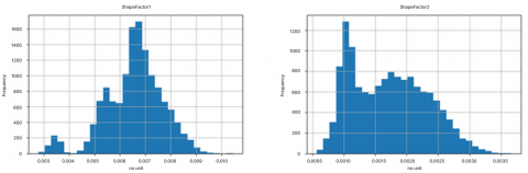
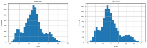
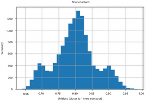
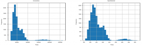
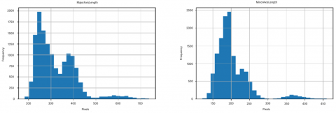
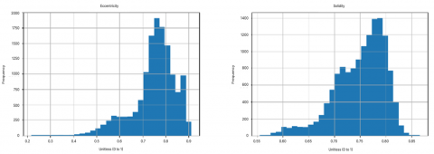
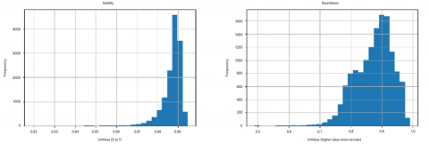
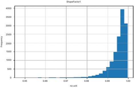
Then, we attach the histogram image of each column in the dataset apart from the Class column, as shown in the Figure 2.
There is information obtained, namely that the ShapeFactor1, ShapeFactor2, ShapeFactor3, AspectRation and Compactness columns have normal distribution values which have symmetrical skewness. This indicates that the data is spread evenly without a strong tendency in a particular direction. This means that the mean, median and mode have the same value and the data is easy to analyze using common statistical methods. The result is shown in the Figure 3.
Table 5. Data type of each column [27]
|
No. |
Column |
Data Type |
|
1 |
Area |
Integer |
|
2 |
Perimeter |
Float |
|
3 |
MajorAxisLength |
Float |
|
4 |
MinorAxisLength |
Float |
|
5 |
AspectRation |
Float |
|
6 |
Eccentricity |
Float |
|
7 |
ConvexArea |
Integer |
|
8 |
EquivDiameter |
Float |
|
9 |
Extent |
Float |
|
10 |
Solidity |
Float |
|
11 |
Roundness |
Float |
|
12 |
Compactness |
Float |
|
13 |
ShapeFactor1 |
Float |
|
14 |
ShapeFactor2 |
Float |
|
15 |
ShapeFactor3 |
Float |
|
16 |
ShapeFactor4 |
Float |
|
17 |
Class |
Object |
The positively skewed distribution information obtained is that the Area, Perimeter, ConvexArea, EquivDiameter, MajorAxisLength and MinorAxisLength columns have positive skewness. This indicates that the data distribution tends to the right because the average value is higher in the right direction of the data distribution. This means that the data is not normally distributed and the average value is greater than the median and mode, so it has to be careful when using general statistical methods.
There is information obtained, namely that the Eccentricy, Extent, Solidity, Roundness and ShapeFactor4 columns have negative skewness. This indicates that the data distribution tends to the left because the average value is higher in the left direction of the data distribution. The data is not normally distributed, and the mean value is smaller than the median and mode, so it has to be careful when using general statistical methods (Figure 4).
Figure 2. Histogram ShapeFactor1, ShapeFactor2, ShapeFactor3, AspectRation, Compactness
Figure 3. Positively skewed distribution
Figure 4. Histogram eccentricity, extent, solidity, roundness, ShapeFactor4
3.4 Class imbalance assessment
The 'Bombay' class had the highest representation, while other classes, such as 'Sira', were underrepresented. To address this imbalance, we applied techniques such as random oversampling of the minority classes and under sampling of the majority class during the training process. This method aimed to create a more balanced training dataset, ensuring that the classifiers would not be biased towards the more prevalent classes. Additionally, we monitored the performance metrics, such as precision, recall, and F1-score, for each class to evaluate how well the models performed across all nut types.
3.5 Training data using SVM
The training data and testing data were separated by 80% and 20%. A model will be created using the SVM method, as shown in the Figure 5.
Figure 5. SVM model
After the separation was carried out, the data that would be trained to form the model was 10,888 and the data used for testing was 2723. The SVM model was trained using the Radial Basis Function (RBF) kernel, which is particularly effective for non-linear classification problems. To optimize the model, we employed hyperparameter tuning using Grid Search to find the best values for the regularization parameter (C) and the kernel coefficient (gamma). Specifically, we tested C values in the range of 0.1 to 10 and gamma values from 0.01 to 1. The best combination was selected based on cross-validation accuracy, ensuring that the model was well-tuned to the dataset. Additionally, a stratified k-fold cross-validation with 10 folds was implemented to maintain the class distribution in each fold, providing a robust assessment of the model's performance.
3.6 Testing data using SVM
At this stage, testing data uses a model that has been trained in the data training process but uses data that has never been used at all, as shown in the Figure 6.
Figure 6. Prediction result of testing data
3.7 Training data using LDA
At this stage, a model will be created using the LDA method, as shown in the Figure 7.
Figure 7. LDA model
For the LDA model, the training process involved calculating the mean vectors and covariance matrices for each class in the training dataset. Prior to training, we confirmed that LDA assumptions, such as data normality and equal class covariance, were met using exploratory data analysis. Additionally, the number of projection components was set to the standard value of one less than the total number of classes, optimizing the model's ability to distinguish between classes. The LDA model was tested using the same 80/20 training and testing split as the SVM model, ensuring a consistent and fair comparison between the two approaches.
3.8 Testing data using LDA
At this stage, testing data uses a model that has been trained in the data training process but uses data that has never been used at all, as shown in the Figure 8.
Figure 8. Prediction result of LDA model
3.9 Discussion
To ensure the reliability and stability of the results, multiple experiments were performed using both the SVM and LDA models. Each model was trained and tested on 10 different random splits of the dataset, and the average accuracy along with other performance metrics was computed across these iterations to ensure a comprehensive evaluation.
Additionally, we analyze feature importance to identify the key characteristics of dry nuts that contributed to accurate classification. For the SVM model, the feature contributions were assessed using the coefficients of the decision boundary, while for the LDA model, we examined the weights assigned to features in the linear discriminant functions. The results showed that features such as 'Area', 'Perimeter', and 'MajorAxisLength' were the most significant in distinguishing between different nut types. This indicates that geometric properties play a critical role in classification. Highlighting feature importance not only improves the interpretability of the models but also offers valuable insights for enhancing data collection and feature engineering in future studies.
3.10 Confusion matrix
The final step is to measure the accuracy of the model that has been developed using the confusion matrix. The formula for calculating accuracy with the confusion matrix is as follows: Accuracy = $\frac{\mathrm{TP}+\mathrm{TN}}{\mathrm{TP}+\mathrm{TN}+\mathrm{FP}+\mathrm{FN}} * 100 \%$ [30].
The results are shown in Figures 9-22.
Figure 9. The result of class Barbunya SVM model
$\begin{gathered}\text { Accuracy }=\frac{240+2445}{240+2445+17+21} * 100 \% \\ \text { Accuracy }=98 \%\end{gathered}$
Figure 10. The result of class Bombay SVM model
$\begin{gathered}\text { Accuracy }=\frac{117+2606}{117+2606+0+0} * 100 \% \\ \text { Accuracy }=100 \%\end{gathered}$
Figure 11. The result of class Cali SVM model
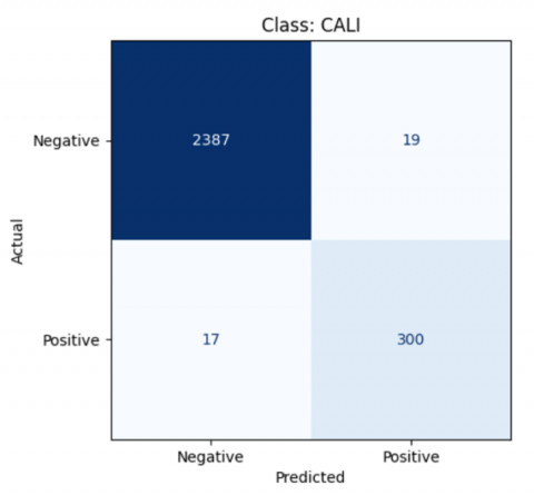
$\begin{gathered}\text { Accuracy }=\frac{300+2387}{300+2387+19+17} * 100 \% \\ \text { Accuracy }=98 \%\end{gathered}$
Figure 12. The result of class Dermason SVM model
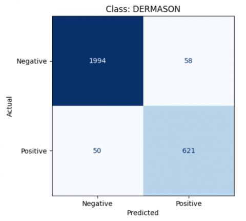
$\begin{gathered}\text { Accuracy }=\frac{621+1994}{621+1994+58+50} * 100 \% \\ \text { Accuracy }=96 \%\end{gathered}$
Figure 13. The result of class Horoz SVM model
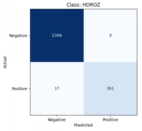
$\begin{gathered}\text { Accuracy }=\frac{391+2306}{391+2306+9+17} * 100 \% \\ \text { Accuracy }=99 \%\end{gathered}$
Figure 14. The result of class Seker SVM model
$\begin{gathered}\text { Accuracy }=\frac{393+2298}{393+2298+12+20} * 100 \% \\ \text { Accuracy }=98 \%\end{gathered}$
Figure 15. The result of class Sira SVM model
$\begin{gathered}\text { Accuracy }=\frac{481+2122}{481+2122+65+55} * 100 \% \\ \text { Accuracy }=95 \%\end{gathered}$
Figure 16. The result of class Barbunya LDA model
$\begin{gathered}\text { Accuracy }=\frac{217+2453}{240+2445+9+44} * 100 \% \\ \text { Accuracy }=98 \%\end{gathered}$
Figure 17. The result of class Bombay LDA model
$\begin{gathered}\text { Accuracy }=\frac{117+2606}{117+2606+0+0} * 100 \% \\ \text { Accuracy }=100 \%\end{gathered}$
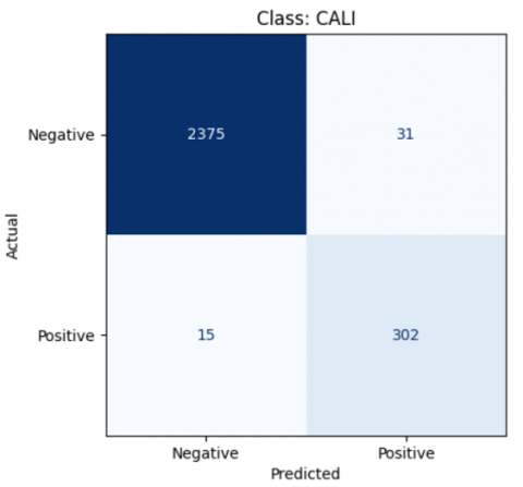
Figure 18. The result of class Cali LDA model
$\begin{gathered}\text { Accuracy }=\frac{302+2375}{302+2375+31+15} * 100 \% \\ \text { Accuracy }=98 \%\end{gathered}$
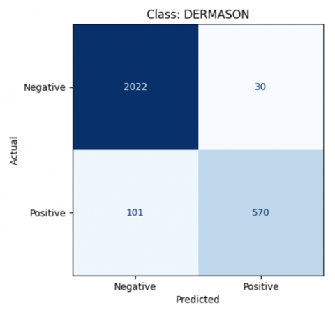
Figure 19. The result of class Dermason LDA model
$\begin{gathered}\text { Accuracy }=\frac{570+2022}{570+2022+30+101} * 100 \% \\ \text { Accuracy }=95 \%\end{gathered}$
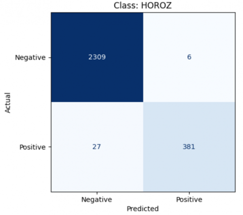
Figure 20. The result of class Horoz LDA model
$\begin{gathered}\text { Accuracy }=\frac{381+2309}{381+2309+6+27} * 100 \% \\ \text { Accuracy }=98 \%\end{gathered}$
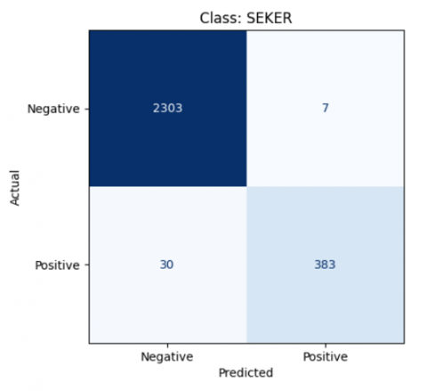
Figure 21. The result of class Seker LDA model
$\begin{gathered}\text { Accuracy }=\frac{383+2303}{383+2303+7+30} * 100 \% \\ \text { Accuracy }=98 \%\end{gathered}$
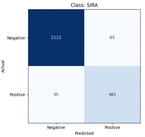
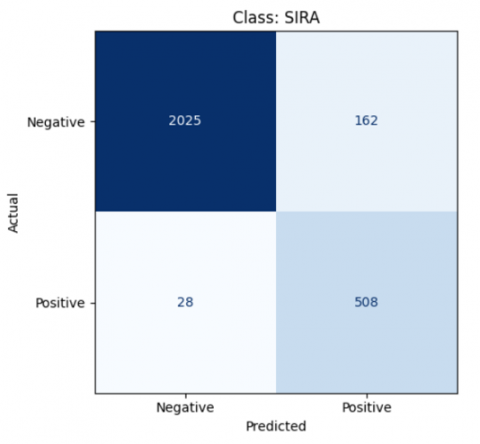
Figure 22. The result of class Sira LDA model
$\begin{gathered}\text { Accuracy }=\frac{508+2025}{508+2025+162+28} * 100 \% \\ \text { Accuracy }=93 \%\end{gathered}$
Following the evaluation of the confusion matrix, we conducted a detailed analysis of misclassifications to understand which types of nuts were most frequently confused by the models. The confusion matrices for both SVM and LDA indicated that certain nut types, such as 'Barbunya' and 'Dermason', were often misclassified as 'Seker'. This pattern suggests that these nuts may exhibit similar geometric characteristics, leading to confusion during classification. Hypothetically, factors such as slight variations in colour, shape, or size, which may not be adequately captured in the features used for modeling, could contribute to these misclassifications. Additionally, the similarities in texture or visual features between these nut types may also play a role in their frequent confusion.
In our analysis of misclassified samples, we observed that the misclassifications were not uniformly distributed across all classes. For example, a notable number of samples from the 'Sira' class were misclassified as 'Dermason'. This could be attributed to the similarity in their geometric features and possibly their size. Moreover, the confusion matrices showed that the model struggled to accurately classify samples from classes with fewer instances, such as 'Sira', leading to higher misclassification rates for these types. This highlights the impact of class imbalance on model performance, where models may not learn adequately about underrepresented classes. Future work could focus on exploring advanced techniques like synthetic data generation for minority classes to mitigate these issues.
From the research conducted on dry nut classification using the SVM and LDA algorithms, the following conclusions have been derived:
(1) There are seven types of dry nut with seven different levels of accuracy based on calculations per class using the SVM and LDA methods.
(2) The results of the accuracy of the SVM method are Barbunya at 98%, Bombay at 100%, Cali at 98%, Dermason at 96%, Horoz at 99%, Seker at 98%, Sira at 95% while the results of the accuracy of the LDA method are Barbunya by 98%, Bombay by 100%, Cali by 98%, Dermason by 95%, Horoz by 98%, Seker by 98%, Sira by 93%.
(3) SVM's ability to handle non-linear data, resistance to outliers, maximum margins, and its ability to work with high-dimensional data make SVM better than LDA for classifying several types of dry beans, namely Dermason, Horoz, and Sira.
This research presents several innovations, including the application of advanced machine learning techniques (SVM and LDA) for the classification of dry nuts, which have not been extensively explored in the agricultural domain. Additionally, the study highlights the importance of feature importance analysis, which provides valuable insights into the characteristics that significantly influence classification accuracy. The incorporation of strategies to address class imbalance through random oversampling and under sampling techniques has also enhanced model performance.
Future research directions may include exploring more sophisticated methods such as deep learning algorithms to further improve classification accuracy and robustness. Additionally, integrating more diverse datasets with enhanced feature extraction methods could yield better insights into the classification of nut types. Investigating the impact of external factors such as environmental conditions on nut characteristics and incorporating these variables into the modeling process could also provide more comprehensive results. Lastly, further studies could focus on the development of real-time classification systems for practical applications in the agricultural sector, enhancing efficiency in the classification and sorting processes.
[1] Yang, B., Chen, H., Chen, W., Chen, W., Zhong, Q., Zhang, M., Pei, J. (2023). Edible quality analysis of different areca nuts: Compositions, texture characteristics and flavor release behaviors. Foods, 12(9): 1749. https://doi.org/10.3390/foods12091749
[2] Amran, A.A., On, C.K., Karim, S.A.A., Hung, L.P., See, C.S., Simon, D., Rossdy, M., Jing, C. (2024). Bornean orangutan nest classification using image enhancement with convolutional neural network and kernel multi support vector machine classifier. Journal of Advanced Research in Applied Sciences and Engineering Technology, 49(2): 187-204. https://doi.org/10.37934/araset.49.2.187204
[3] Yang, S.F., Jia, Z.C., Yi, K., Zhang, S.H., Zeng, H.G., Qiao, Y., Mao, P.S., Li, M.L. (2024). Rapid prediction and visualization of safe moisture content in alfalfa seeds based on multispectral imaging technology. Industrial Crops and Products, 222: 119448. https://doi.org/10.1016/j.indcrop.2024.119448
[4] Kaveripakam, D., Ravichandran, J. (2025). Comparative analysis of machine learning algorithms for diabetic disease identification. Journal of Advanced Research in Applied Sciences and Engineering Technology, 45(1): 40-50. https://doi.org/10.37934/araset.45.1.4050
[5] Yildiz, E.P., Coskun, O., Kurekci, F., Genc, H.M., Ozaltin, O. (2024). Machine learning models for predicting treatment response in infantile epilepsies. Epilepsy & Behavior, 160: 110075. https://doi.org/10.1016/j.yebeh.2024.110075
[6] Heednacram, A., Kliangsuwan, T., Werapun, W. (2024). Implementation of four machine learning algorithms for forecasting stock’s low and high prices. Neural Computing and Applications, 36(31): 19323-19336. https://doi.org/10.1007/s00521-024-10247-6
[7] Nguyen, M., Nguyen, B., Liêu, M.L. (2024). Corporate financial distress prediction in a transition economy. Journal of Forecasting. 43(8): 3128-3160. https://doi.org/10.1002/for.3177
[8] Damayanti, N.P., Puspita, W., Sundari, P.S. (2024). The classification of hate comments on Twitter using a combination of logistic regression and support vector machine algorithm. Journal of Information System Exploration and Research, 2(1): 49-60. https://doi.org/10.52465/joiser.v2i1.229
[9] Jin, Z., Wang, T., Luo, Z. (2025). Wire rope damage detection method based on support vector machine wavelet kernel function algorithm. Communications in Computer and Information Science, 2183: 284-298. https://doi.org/10.1007/978-981-97-7007-6_20
[10] Zhong, W., Du, L. (2023). Predicting traffic casualties using support vector machines with heuristic algorithms: A study based on collision data of urban roads. Sustainability, 15(4): 2944. https://doi.org/10.3390/su15042944
[11] Zhang, H., Zou, Q., Ju, Y., Song, C., Chen, D. (2022). Distance-based support vector machine to predict DNA N6-methyladenine modification. Current Bioinformatics, 17(5): 473-482. https://doi.org/10.2174/1574893617666220404145517
[12] Zhang, L., Li, C., Chen, L., Chen, D., Xiang, Z., Pan, B. (2023). A Hybrid forecasting method for anticipating stock market trends via a soft-thresholding de-noise model and support vector machine (SVM). World Basic and Applied Sciences Journal, 13(2023): 597-602
[13] Al-Khowarizmi, Sari, I.P., Halim, M. (2023). Detecting cyberbullying on social media using support vector machine: A case study on Twitter. International Journal of Safety and Security Engineering (IJSSE), 13(4): 709-714. https://doi.org/10.18280/ijsse.130413
[14] Abdallah, A.A., Abdallah, M.S.E.S., Aslan, H., Azer, M.A., Cho, Y.I., Abdallah, M.S. (2024). Enhancing Mobile Ad Hoc Network security: An anomaly detection approach using support vector machine for black-hole attack detection. International Journal of Safety and Security Engineering (IJSSE), 14(4): 1015-1028. https://doi.org/10.18280/ijsse.140401
[15] Farrar, M.B., Omidvar, R., Nichols, J., Pelliccia, D., Al-Khafaji, S.L., Tahmasbian, I., Hapuarachchi, N., Bai, S.H. (2024). Hyperspectral imaging predicts macadamia nut-in-shell and kernel moisture using machine vision and learning tools. Computers and Electronics in Agriculture, 224: 109209. https://doi.org/10.1016/j.compag.2024.109209
[16] Adebiyi, M.O., Arowolo, M.O., Mshelia, M.D., Olugbara, O.O. (2022). A linear discriminant analysis and classification model for breast cancer diagnosis. Applied Sciences, 12(22): 11455. https://doi.org/10.3390/app122211455
[17] Abusham, E., Ibrahim, B., Zia, K., Rehman, M. (2023). Facial image encryption for secure face recognition system. Electronics, 12(3): 774. https://doi.org/10.3390/electronics12030774
[18] Hadiyoso, S., Wijayanto, I., Humairani, A. (2023). Entropy and fractal analysis of EEG signals for early detection of alzheimer's dementia. Traitement du Signal (TS), 40(4): 1673-1679. https://doi.org/10.18280/ts.400435
[19] Olaniyi, E., Kucha, C., Dahiya, P., Niu, A. (2024). Precision variety identification of shelled and in-shell pecans using hyperspectral imaging with machine learning. Infrared Physics & Technology, 142: 105570. https://doi.org/10.1016/j.infrared.2024.105570
[20] Pratama, I.P.A., Atmadji, E.S.J., Purnamasar, D.A., Faizal, E. (2024). Evaluating the performance of voting classifier in multiclass classification of dry bean varieties. Indonesian Journal of Data and Science, 5(1): 23-29. https://doi.org/10.56705/ijodas.v5i1.124
[21] Khan, M.S., Nath, T.D., Hossain, M.M., Mukherjee, A., Hasnath, H.B., Meem, T.M., Khan, U. (2023). Comparison of multiclass classification techniques using dry bean dataset. International Journal of Cognitive Computing in Engineering, 4(2023): 6-20. https://doi.org/10.1016/j.ijcce.2023.01.002
[22] Guerrero, M.C., Parada, J.S., Espitia, H.E. (2021). EEG signal analysis using classification techniques: Logistic regression, artificial neural networks, support vector machines, and convolutional neural networks. Heliyon, 7(6): 1-19. https://doi.org/10.1016/j.heliyon.2021.e07258
[23] Shahoveisi, F., Riahi Manesh, M., del Río Mendoza, L.E. (2022). Modeling risk of Sclerotinia sclerotiorum-induced disease development on canola and dry bean using machine learning algorithms. Scientific Reports, 12(1): 864. https://doi.org/10.1038/s41598-021-04743-1
[24] Laraswati, B. (2022). Mengenal kelemahan dan kelebihan naive bayes. https://blog.algorit.ma/kelebihan-naive-bayes/.
[25] DQLab. (2023). Serba serbi machine learning model random forest. https://dqlab.id/serba-serbi-machine-learning-model-random-forest.
[26] Bejani, M.M., Ghatee, M. (2021). A systematic review on overfitting control in shallow and deep neural networks. Artificial Intelligence Review, 54: 6391-6438. https://doi.org/10.1007/s10462-021-09975-1
[27] Koklu, M., Ozkan, I.A. (2020). Multiclass classification of dry beans using computer vision and machine learning techniques. Computers and Electronics in Agriculture, 174: 105507. https://doi.org/10.1016/j.compag.2020.105507
[28] Ahmed, N., Khan, F.A., Ullah, Z., Ahmed, H., Shahzad, T., Ali, N. (2021). Face recognition comparative analysis using different machine learning approaches. Advances in Science and Technology. Research Journal, 15(1): 265-272. https://doi.org/10.12913/22998624/132611
[29] UCI Machine Learning Repository. (2020). Dry Bean Dataset. https://doi.org/10.24432/C50S4B
[30] Zeng, G. (2020). On the confusion matrix in credit scoring and its analytical properties. Communications in Statistics-Theory and Methods, 49(9): 2080-2093. https://doi.org/10.1080/03610926.2019.1568485