Shivali Amit Wagle![]() | R Harikrishnan*
| R Harikrishnan*![]() | Ketan Kotecha
| Ketan Kotecha![]()
© 2024 The authors. This article is published by IIETA and is licensed under the CC BY 4.0 license (http://creativecommons.org/licenses/by/4.0/).
OPEN ACCESS
Climate change threatens agriculture; as a result, adaptation measures are required to withstand agricultural produce, reduce susceptibility, and improve the farm system's flexibility to climate change. Meteorological parameters like temperature and relative humidity play an essential role in the condition of disease occurrence in plants. We studied ARIMA, Prophet, and Long Short-Term Memory (LSTM) with stochastic gradient descent with momentum, RMSprop, and Adam optimizers to forecast the temperature and relative humidity. The work proposes a hybrid regression prediction model of Bilinear LSTM with Gaussian Bayesian optimization (BLSTM_bayOpt) for predicting disease in tomato plants based on weather parameters. From the six prediction models in this study, the performance of BLSTM_bayOpt in prediction with RMSE of 1.1573 and 5.5509, MAPE is 0.0556 and 0.0927, R2 is 0.9324 and 0.9475 for temperature and relative humidity, respectively. The proposed hybrid BLSTM_bayOpt model improved by 40.67%, with an MSE score for relative humidity prediction.
Bayesian optimization, long short-term memory, prediction, relative humidity, temperature, tomato plant disease
In terms of total area and tomato production, India contributes approximately 19.0 and 11.1%, respectively, to the global total. Tomatoes account for 8% and 12% of total vegetable cultivation area and production in India, respectively [1]. Predicting disease and timely management can help reduce the loss in yield and help farmers produce better. Weather factors such as “temperature, rainfall, leaf wetness duration, and relative humidity” are driving factors in plant disease forecasting. Hourly or daily data is essential for weather-driven models to detect infection conditions and track disease cycles [2]. Weather forecasting is a critical area of study in everyday life. Weather for the future is essential to forecast because agriculture and many industries rely heavily on weather conditions. Weather forecasting is required for future planning in agriculture, industry, and other fields such as defence, mountaineering, shipping, aerospace navigation, etc. [3-6]. Weather forecasting involves the application of scientific principles and advanced technology to predict the atmospheric conditions at a particular place and time in the future. These forecasts rely on the dynamic nature of various factors such as temperature (both high and low), relative humidity, and precipitation, among others, as they constantly fluctuate over time [7]. For developing a forecasting model, a time series for each parameter can be formed statistically [8]. Various approaches have been developed for weather forecasting and statistical analysis in the past decades. Regression models are still widely used approaches for predicting future events or values in these models [9, 10].
The time-series weather data consists of various parameters viz temperature, humidity, dewpoint, rainfall, and wind speed information on an hourly, daily, and weekly format. Numerous profound learning architectures have been designed to diversify data series in different fields [11]. The various models are linear regression, support vector regression, random forest regression, “Auto-Regressive Integrated Moving Average” (ARIMA), “Seasonal Autoregressive Integrated Moving Average” (SARIMA), Prophet, Convolutional Neural Networks (CNN), Recurrent Neural Networks Recurrent (RNN), Long Short-term Memory (LSTM) to name a few that can be applied to a time-series data. In predicting plant disease, time-series weather data analysis must be done for weather parameters like temperature and relative humidity that cause favorable environmental conditions for the disease triangle [12]. The hybrid model might give a better forecast result in the weather prediction that can predict disease occurrence in plants in advance. The hybrid model can use post-processing techniques like model output statistics to improve the prediction handling errors with optimization methods [13, 14]. The prediction of tomato plant leaves disease occurring at a particular temperature and relative humidity is discussed in this work.
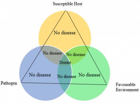
1.1 Disease triangle
The plant disease triangle offers a lens through which we understand that the occurrence of a plant disease arises from the intricate interplay between a pathogen, a host, and the environment, highlighting the dynamic and multifaceted nature of these interactions [15, 16]. Plant disease prediction systems can aid farmers in averting diseases by providing early detection and alerting them when their crops are susceptible to infection. It is critical to have a mechanism for anticipating plant diseases.
Figure 1. The dynamics of plant disease through disease triangle
The approach anticipates the potential for plant infections triggered by environmental conditions that facilitate germination [17]. Factors such as temperature, relative humidity, absolute humidity, and rainfall are pivotal in fostering an environment favorable for plant diseases. These non-living elements profoundly influence the variation in pest populations [18]. The disease triangle, as depicted in Figure 1, results in disease in plants.
Under these circumstances, plant infection occurs only when there is a conducive environmental condition for the pathogen to thrive and the host plant to be susceptible [19]. A low-level disease in most plants is common, but sporadic epidemics can unacceptably decrease cultivation quality or yield. Genetic resistance in the host plant can sometimes prevent plant disease epidemics. Farmers often have to depend on the prudential use of crop guards in terms of chemical substances to prevent conditions from getting severe enough to have an economic impact on quality and yield without genetic resistance [20].
This work emphasizes deep learning techniques to predict tomato plant disease (TPD) in the Pune region.
Our contribution is as follows:
(1) A hybrid Bilinear Long Short-term Memory (BLSTM) model with Bayesian optimization for temperature and relative humidity prediction.
(2) ARIMA, Prophet, and LSTM models with stochastic gradient descent with momentum (SGDM), RMSprop, and Adam optimizers models have been used on the dataset to forecast the temperature and relative humidity.
(3) A comparative analysis of different deep learning models is discussed.
(4) Prediction of temperature and relative humidity helps in predicting.
The paper is arranged as follows. Section 2 provides related work on prediction models and plant disease prediction. The proposed method is presented in Section 3. The results and discussion of the study are in Section 4. The conclusion and suggestions for future work are in Section 5.
In predicting the power load for the American Electric power dataset, Jin et al. [13] used a decomposition model. The performance of the model was improved with the Bayesian optimization. The BLSTM-GRU model was used to predict rainfall in Simtokha, Bhutan, which increased 41.1% performance in MSE value compared to the LSTM model [21]. After Bayesian optimization, the season-wise prediction of photovoltaic power was improved with the LSTM-attention embedding [22]. In predicting air temperature for the Bandung region, the Prophet model performed well with an RMSE of 1.03 compared to the RMSE of 1.23 for the LSTM model [23].
A Spatio-temporal recurrent neural network was used by Xu et al. [24] to predict wheat crop disease severity. The prediction of leaf wetness duration also causes disease in plants. In the study of Wang et al. [25], they collected the greenhouse data of tomato plants from Almeria, Spain, and Beijing, China that predicted relative humidity, dew temperature, transpiration, radiation, and a combination of all these factors. A neural network simulator was used for the prediction of parameters. The relative humidity was predicted with 73% and 83% accuracy in Spain and China's greenhouse data, respectively. The overall performance was 82% and 98% for the Spain and China datasets, respectively. For seasonally repeated patterns, statistical regression models like Prophet are used [26]. In Myintkyina, Malaysia, Temperature prediction was done by Oo and Sabai [27] with the Prophet model that gave the RMSE value of 5.7573.
The Pusa Ruby variety of tomato plants was considered to study the occurrence of early blight in the plants by the study of Gupta et al. [1]. The disease intensity was evaluated with the temperature and relative humidity values. They achieved the performance of the stepwise regression model with an RMSE of 6.129 for the prediction of disease intensity. Dar et al. [28] used a stepwise regression model to predict late blight in potato plants for the four potato varieties. The parameters of temperature, relative humidity, rainfall, and windspeed were considered for disease prediction. Table 1 shows the comparative study of a prediction model for disease occurrence.
Farmers can have more tools for disease control strategies if weather forecast data is used for disease warnings. With the help of forecast data, farmers can be able to use a pre-infection treatment like the use of protective fungicides and cultural practices. In terms of suppressing fungicide resistance and cost efficiency, pre-infection therapies demonstrate greater effectiveness in plants compared to post-infection treatments. The advantages of utilizing weather prediction data are evident in predicting plant diseases. However, there is a scarcity of research focused on utilizing weather prediction models for managing pests and diseases [2]. Better disease management can be availed through a weather-driven disease prediction model, and weather prediction data would be a tremendous facilitator in the application.
The methodology to predict the occurrence of TPD based on the prediction of meteorological parameters like temperature and relative humidity using the deep learning approach is discussed in the next section.
Table 1. Comparative study of a prediction model for the occurrence of disease
|
Ref |
Main Idea |
Performance |
Dataset |
Limitations |
|
[24] |
Prediction of the wheat crop disease |
The RMSE was improved to 0.0740 |
Weather data of Longnan City, China |
Fine-tuning of models can be done for performance improvement |
|
[25] |
Evaluation of leaf wetness duration |
Relative humidity prediction is 73% in Spain and 83% in China |
Greenhouse data from Almeria, Spain, and Beijing, China |
Experiments were performed on greenhouse data |
|
[1] |
Prediction of the intensity of early blight disease in tomato |
The disease intensity RMSE value is 6.129 |
Weather data of Jammu province, India |
Only one class of Pusa Ruby was considered for the study |
|
[27] |
Temperature Forecasting in Myintkyina |
RMSE is 5.7573 |
Temperature data of Myintkyina |
High computational cost |
|
[28] |
Prediction of temperature and relative humidity for disease in Sorghum |
Validation of disease at two different locations shows good performance. |
Weather parameters of Ludhiana, India |
Models can be explored for other zones for the prediction of disease |
|
[29] |
Prediction of late blight disease in potato |
RMSE of 0.58 for Kufri Jyoti variety |
Weather parameters of Kashmir, India |
The study was carried out for hilly regions only |
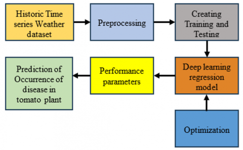
The workflow for the proposed study in predicting TPD is shown in Figure 2. A historic time-series dataset of environmental parameters is selected for the Pune region [30]. The dataset is pre-processed and divided into training and testing datasets before applying a deep-learning regression model. The performance of the deep learning model is evaluated, and the prediction of the occurrence of disease in tomato plants is made.
Figure 2. Workflow of the proposed work in the TPD prediction
3.1 Dataset
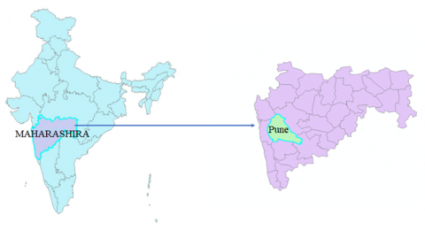
By leveraging time-series data, the analysis facilitates continuous tracking of weather patterns at varying daily, hourly, or weekly intervals. The investigation utilizes a comprehensive weather dataset sourced from the Pune region in Maharashtra state, India, covering observations from January 1, 2009, to January 1, 2020 [30]. Figure 3, depicts the geographical area of Pune in Maharashtra, India, this specific region was selected as the focal point for the research. The dataset encompasses diverse meteorological variables including maximum and minimum temperatures, humidity, rainfall, dewpoint, wind speed, and wind direction.
According to the principles outlined in the disease triangle, conducive weather conditions play a pivotal role in nurturing pathogens, thereby contributing to plant diseases. Particularly in the case of tomato plants, the relative humidity emerges as a crucial factor in influencing favorable conditions for disease development [31]. The calculation of relative humidity, as described in Eq. (1), involves determining the ratio between saturated vapor pressure and actual vapor pressure.
Figure 3. Geographical positioning of the Pune region in Maharashtra, India, for the weather dataset collection
Relative Humidity $=\frac{E}{E_s} X 100$ (1)
where,
saturated vapor pressure $(E)$$=6.11 \times 10^{\Lambda}\left(\frac{7.5 \text { Xdewpoint }}{237.7+\text { dewpoint }}\right)$
and
Actual vapor pressure $\left(E_s\right)$$=6.11 \times 10^{\Lambda}\left(\frac{7.5 X \text { Temperature }}{237.7+\text { Temperature }}\right)$
Prior to commencing the analysis, the dataset underwent a pre-processing stage aimed at detecting and handling any missing data entries. The weather forecasting analysis specifically focused on essential weather parameters such as temperature, dewpoint, pressure, relative humidity, and absolute humidity. To facilitate the analysis, the dataset was divided into separate training and testing sets, with an 80% portion allocated for training and the remaining 20% for testing.
3.2 Deep learning models
Artificial Intelligence-based algorithms are used for complex regression models. Regression was used to detect the complex correlation between input and output variables [32]. In our study, we leverage various advanced models-Auto-Regressive Integrated Moving Average (ARIMA), Facebook Prophet, Long Short-Term Memory (LSTM) employing three different optimizers, and Bilinear LSTM using Bayesian optimization-to forecast both temperature and relative humidity. As these parameters are crucial in the occurrence of TPD, the forecast will help get a solution for managing plants in those weather conditions. ARIMA models were selected due to their effectiveness in modeling linear dependencies in time-series data. Its ability to capture trends, seasonality, and stationarity in the context of plant disease progression was a primary consideration [33]. The prophet model can handle seasonal data with irregularities by capturing varied patterns that traditional statistical models might not fully [34]. LSTM was employed for its capacity to model complex temporal relationships and nonlinear dependencies within the data [35]. the integration of Bayesian optimization was pivotal in fine-tuning hyperparameters for these models, optimizing their performance, and overcoming challenges related to parameter tuning, thereby enhancing their predictive accuracy [36].
3.2.1 ARIMA
A famous time series prediction method introduced by Box and Jenkins is ARIMA. The main formulas of ARIMA are as follows: Prediction of future values can be made with the combination of auto-regression and moving average algorithms in ARIMA. ARIMA models can handle stationary and non-stationary time series. Data autocorrelation patterns are essential in ARIMA. ARIMA's methodology differs because it uses an interactive approach to identify a possible model [37]. ARIMA (p, d, q) captures the model's essential elements: “autoregressive, integrated, and moving average.” “The time series is linearly dependent on its preceding values and a stochastic term, as per the autoregressive (AR) process. The model of order p forecasts the variable when there is a correlation between the time series value and its predecessors” [38, 39].
$Y_t=c+\alpha_1 Y_{t-1}+\alpha_2 Y_{t-2}+\cdots+\alpha_p Y_{t-p}+\epsilon_t$ (2)
The integration process (I) is employed to achieve stationarity in time series by assessing the differences between observations made at various points in time (d). In utilizing a Moving Average (MA) model applied to past observations, this approach considers the relationship between observations and residual error terms (q) [39].
$Y_t=\epsilon_t+\theta_1 \epsilon_{t-1}+\theta_2 \epsilon_{t-2}+\cdots+\theta_q \epsilon_{t-q}$ (3)
where, " $Y_t$ represents the stationary variable. 'c' denotes the constant term, while the $\alpha_p$ and $\theta_q$ terms stand for autocorrelation coefficients ranging from lag 1 to $\mathrm{N}$. Additionally, $\epsilon_t$ is the stochastic term". ARIMA has three parameters: "autoregressive order (p), differencing degree (d), and moving average order (q)." The ARIMA (p, d, q) model is written as follows:
$\begin{gathered}\Delta Y_t=c+\alpha_1 \Delta Y_{t-1}+\cdots+\alpha_p \Delta Y_{t-p}+\epsilon_t+\theta_1 \epsilon_{t-1} \\ +\theta_2 \epsilon_{t-2}+\cdots+\theta_q \epsilon_{t-q}\end{gathered}$ (4)
Augmented Dickey and Fuller test is performed to identify the time series data into a stationary or not category [38]. Variance-stabilizing transformations and differencing are used for the time series plots showing variance growth. To determine the amount of linear dependence between observations in a time series separated by a lag p, Autocorrelation Function (ACF) is used. The number of autoregressive terms q is determined by the Partial Autocorrelation Function (PACF). Inverse Autocorrelation function (IACF) can identify preliminary autoregressive order p, order of differencing d, and moving average order q along with over differencing. The order of difference frequency changing from non-stationary to stationary time series is represented by the parameter d [39]. Estimate relevant models based on the ACF and PACF series, adjusting the level of AR and MA. In ACF and PACF graphs, the spikes and curves help us identify (p, q). Once the optimum model has been picked, forecasting uses the model's parameters (p, d, q). Assessing the performance of the newly built forecasting model involves utilizing statistically significant measures like the Akaike information criterion (AIC), Bayesian information criterion (BIC), and mean square error (MSE). This evaluation process aids in determining the effectiveness and accuracy of the model [38, 40].
3.2.2 Prophet
Prophet is a forecasting model created by Facebook Research, the company's R&D division dedicated to developing innovative solutions. Forecast plays a significant role in a big organization. The organization considers forecasting a crucial tool for planning capacity and efficiently dividing limited resources and goal setting. High-quality forecasts are challenging for machines or analysts [41]. The prophet model utilizes a decomposable time series framework, comprising three key elements-trend, seasonality, and holidays-as components in its prediction of the output variable y(t) [26, 29]:
$y(t)=g(t)+s(t)+h(t)+\varepsilon(t)$ (5)
where, g(t) represents the trend that can be linear or non-linear, s(t) represents the seasonality changes, h(t) represents the holiday information, ε(t) is the error term; this approach is beneficial in many ways.
The seasonal component s(t) offers a versatile representation of cyclical variations arising from weekly and yearly patterns. On the other hand, the h(t) component captures anticipated annual irregularities, accounting for atypical occurrences such as days with irregular schedules. The error term “ε(t) denotes information not expressed in the model.” It is commonly modelled as normally distributed noise.
3.2.3 LSTM
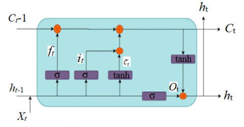
The LSTM proposed by Hochreiter and Schmidhuber is a computing unit in a Recurrent Neural Network (RNN) structure [42]. The LSTM computes data through three gates: a forget gate deals with the removal of data, an input gate deals with the number of cell states stored, and an output gate deals with the cell states to be taken forward [43]. Within the gate mechanism, various terms are employed: $\sigma$ denotes the sigmoid activation function, tanh represents the hyperbolic tangent activation function, $h_{t-1}$ signifies the output of the hidden state at time $\mathrm{t}-1, x_t$ denotes the input at time $\mathrm{t}$, and $\tilde{C}_t$ indicates the intermediary cell state [23]. Figure 4 shows the LSTM model architecture. Several network models are trained at the same time. The best model is one with a minimum amount of error, which can be achieved when each gate function reaches maximum epochs or target error.
Figure 4. LSTM model architecture
The following information is passed through the forget gate, information gate, intermediate cell state, new cell state, output gate, and output for the hidden state is shown in Eq. (6) to Eq. (11):
$f_t=\sigma\left(W_f \cdot\left[h_{t-1}+x_t\right]+b_f\right)$ (6)
$i_t=\sigma\left(W_i \cdot\left[h_{t-1}+x_t\right]+b_i\right)$ (7)
$\tilde{C}_t=\tanh \left(W_c \cdot\left[h_{t-1}+x_t\right]+b_c\right)$ (8)
$c_t=\left(i_t * \tilde{C}_t+f_t * c_{t-1}\right)$ (9)
$o_t=\sigma\left(W_o .\left[h_{t-1}, x_t\right]+b_0\right)$ (10)
$h_t=o_t * \tanh \left(c_t\right)$ (11)
where, $W_f, W_i, W_c$, and $W_o$ are weights and $b_f, b_i, b_c$ and $b_o$ are bias of the forget gate, input gate, output gate, and cell state.
The LSTM model is trained with three optimizers sgdm, RMSprop, and Adam. Adam is a stochastic gradient descent replacement optimization algorithm for deep learning model training. Optimum features of the AdaGrad and RMSProp algorithms are integrated for optimization to deal with sparse gradients on noisy problems. The LSTM layer is further connected to a fully connected layer, followed by a dropout layer, a fully connected layer, and the regression layer for temperature and relative humidity prediction. The dropout layer reduces the overfitting problem [44].
3.2.4 BLSTM-Bayesian optimization
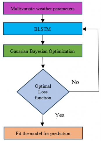
The proposed hybrid model is Bilinear LSTM(BLSTM) with Gaussian Bayesian optimization. The BLSTM model was proposed by Graves and Schmidhuber [45]. In BLSTM, there are two models instead of conventional LSTM The initial model learns from the input sequence provided, while the subsequent model learns from the reverse sequence of the input. After learning the relevant information of each piece in a sequence, current connections are utilized by BLSTM to model the global dependencies amongst their responses internally. It maintains long-term dependence by using specifically designed memory cells [46]. BLSTM is based on the multiplicative interaction of input and LSTM memory [47].
$h_{t-1}=\left[h_{t-1,1}^T, h_{t-1,2}^T, \ldots, h_{t-1, r}^T\right]^T$ (12)
$H_{t-1}^{\text {reshaped }}=\left[h_{t-1,1}, h_{t-1,2}, \ldots, h_{t-1, r}\right]^T$ (13)
$m_t=g\left(H_{t-1}^{\text {reshaped }} x_t\right)$ (14)
where, $g(\cdot)$ is the non-linear activation function. $h_{t-1}$ is a long vector, is reshaped before multiplying it with the input. The matching vector $m_t$ is fed to the fully connected layer and then the dropout layer to avoid overfitting. Gaussian Bayesian optimization is applied to minimize the loss function, and further, the model is fitted for temperature and relative humidity prediction.
Bayesian optimization improves model performance by selecting the best hyperparameters, resulting in a one-of-a-kind optimal model adaptable to each appliance's unique settings and seasonal variations [48]. Behind the Bayesian optimization, the main idea is to start the prior distribution model and then use the data obtained to continuously optimize the guessing model to make it respect the actual distribution. Using the information from the previous sampling point to make it respect the actual distribution can improve the result to maximize the global optimum [49]. The proposed BLSTM model is shown in Figure 5.
Figure 5. BLSTM model architecture
3.3 Performance evaluation
The performance parameters can be evaluated and compared for the different regression models to select the best-performing model. The performance parameter [22] of “Mean Absolute Error (MAE),” “Mean Square Error (MSE),” “Root Mean Square Error (RMSE),” “Coefficient of determination (R2),” and “Mean Absolute Percentage Error (MAPE)” are evaluated for the proposed models for the prediction of temperature and relative humidity as shown in Eq. (15) to Eq. (19). “MAE is a regression loss function which is the mean of the absolute differences between the true and predicted values; deviations from the true value in either direction are treated the same way.” “MSE is a risk function that measures the average squared difference between the estimated and actual values.” RMSE is a popular metric for assessing the accuracy of a model's prediction. “RMSE calculates the differences or residuals between the actual and predicted values.” When predicting the outcome of a given event, the coefficient of determination is a statistical measurement investigating how differences in another variable can explain differences in one variable. “MAPE is a measure of prediction accuracy of a forecasting method in statistics.”
$M A E=\frac{1}{N} \sum_{i=1}^N\left|y_i-\hat{y}\right|$ (15)
$M S E=\frac{1}{N} \sum_{i=1}^N\left(y_i-\hat{y}\right)^2$ (16)
$R M S E=\sqrt{M S E}=\sqrt{\frac{1}{N} \sum_{i=1}^N\left(y_i-\hat{y}\right)^2}$ (17)
$R^2=1-\frac{\sum\left(y_i-\hat{y}\right)^2}{\sum\left(y_i-\bar{y}\right)^2}$ (18)
$M A P E=\frac{1}{N} \sum_{i=1}^N\left|\frac{y_i-\hat{y}}{y_i}\right|$ (19)
$N R M S E=\frac{R M S E}{\max (\text { target })-\min (\text { taget })}$ (20)
Adjusted $R^2=1-\left[\frac{\left(1-R^2\right) X(N-1)}{(N-p-1)}\right]$ (21)
where, $y_i$ is the actual value
$\hat{y}$ is the predicted value of $y_i$
$\bar{y}$ is the mean value of $y_i$
N is the number of observations.
max(target) is maximum value of target variable
min(target) is minimum value of target variable
p is the number of independent variables in the model
3.4 Tomato plant disease
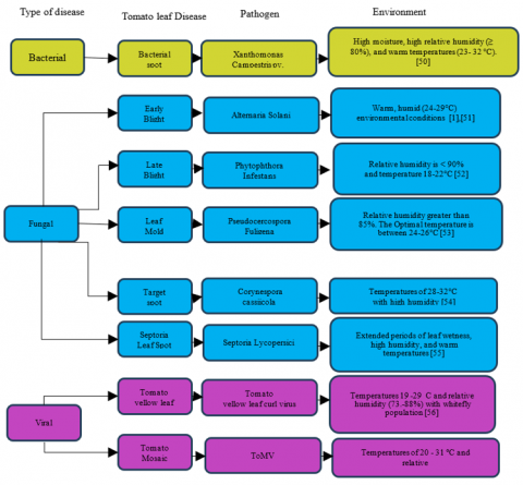
The Optimal conditions for TPD are illustrated in Figure 6, categorizing them as viral, fungal, or bacterial. Environmental factors, including temperature and relative humidity, play crucial roles in the manifestation of eight distinct leaf diseases in tomato plants. Disease occurrence in tomato plants is contingent upon maximum and minimum temperatures, dewpoint, relative humidity, and rainfall. For instance, fungal infections in tomato plants thrive within temperature ranges of 22-38°C and relative humidity levels of 55-90% [50-55]. Conversely, bacterial infections in tomato plants flourish in temperatures ranging from 24-32°C, coupled with relative humidity levels exceeding 80% [56]. The mosaic virus is known to affect tomato plants within temperature ranges of 21-31°C and a relative humidity of 55-70% [57]. Meanwhile, the yellow leaf curl virus manifests when the whitefly population exists between 19-29°C with a relative humidity ranging from 73-88% [58].
Figure 6. Prime environmental settings fostering TPD development
The proposed methodology is applied on the meteorological dataset of Pune region to predict the temperature and relative humidity as theses parameters are very essential to predict the occurrence of disease in plants. The performance parameters are evaluated to study the performance of the proposed model to predict temperature and relative humidity. The results of the prediction are discussed in the following section.
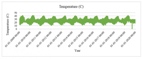
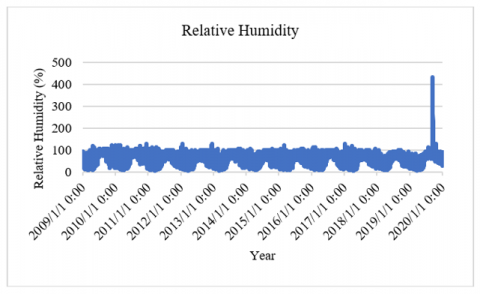
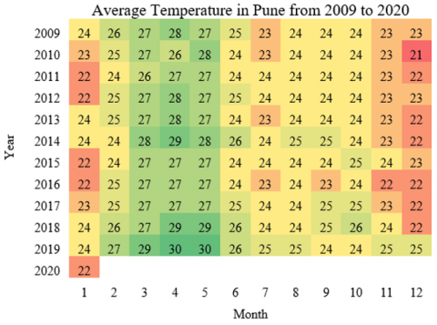
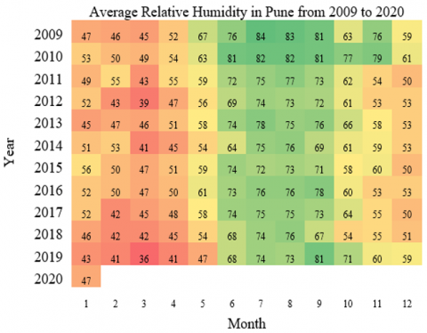
The dataset is found to be clean and has no missing values when checked at the time of preprocessing. Visualizing the fluctuation of parametric values across 11 years of meteorological data illustrates the seasonal patterns within the range [30]. The temperature in degrees Celsius and relative humidity are assessed for the weather forecast. Figure 7 depicts the monthly average temperature in Pune from January 2009 to January 2020. The monthly average relative humidity of Pune for January 2009 to January 2020 is shown in Figure 8. As relative humidity is affected by temperature, outlier temperatures have an effect on relative humidity values.
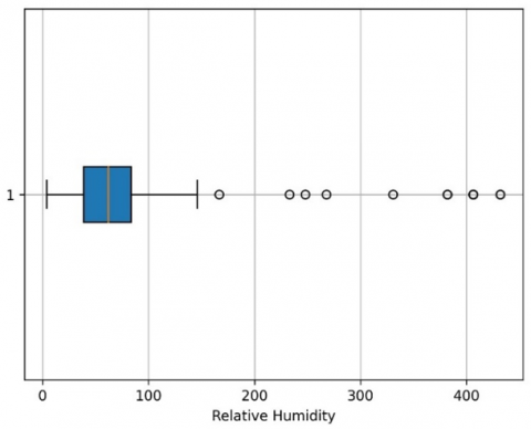
A boxplot helps reveal overall patterns hidden in a dataset and displays a large dataset’s characteristics [59]. Figure 9 displays the boxplot representing the temperature values. Within this plot, certain outlier temperature values exert an influence on the corresponding relative humidity values. Additionally, Figure 10 portrays the boxplot illustrating the relative humidity values.
The average monthly range of temperature values in Pune from January 1 2009 to January 1 2020 is shown in Figure 11. The average monthly temperature is high from March to May every year, which is summer. The average monthly relative humidity for the same period is shown in Figure 12. The relative humidity is higher during the rainy season of June to September every year.
Figure 7. Temperature readings displaying seasonal variation from 2009 to 2020
Figure 8. Relative humidity readings displaying seasonal variation from 2009 to 2020
Figure 9. Boxplot for temperature values
Figure 10. Boxplot for the relative humidity values
Figure 11. Average temperature in Pune
As per the disease triangle, the most favorable environmental conditions responsible for the TPD are majorly dependent on weather parameters viz temperature and relative humidity as shown in Figure 6. So, the temperature and relative humidity are predicted of the prediction of occurrence of TPD. The proposed work V/s other existing works in prediction work is shown in Table 2. The prediction of financial data [39] used ARIMA and LSTM models. In their work, the LSTM model outperformed the ARIMA model. Yang et al. [22] predicted photovoltaic power with LSTM and BLSTM models achieving RMSE of 1.195 and 1.135, respectively. A stepwise regression model was used by Gupta et al. [1] to predict the intensity of tomato early blight disease. They achieved the RMSE of 6.129 and R2 of 0.832. A stepwise regression model with temperature, rainfall, relative humidity, and wind speed was considered to predict potato blight disease [28]. The four varieties of potatoes were chosen for the study. The Kufri Jyoti variety performs best prediction with an RMSE of 0.58 and R2 of 0.82. Bhardwaj et al. [27] used the M1, M2, and M3 models to predict the temperature and relative humidity in the Ludhiana region. The M1 model performed better than the M2 model regarding RMSE and R2 in temperature prediction. The M3 model achieved R2 of 0.12 and RMSE of 12.09 in the prediction of relative humidity. Temperature Forecasting in Myintkyina was done using the Prophet model by Oo and Sabai [26], getting an RMSE of 5.7573. Air temperature forecasting was done by Toharudin et al. [23] using the LSTM model with Adam and RMSProp optimizer and Prophet model. The RMSE of the Prophet model is 1.03, making it a better performer in prediction.
In the proposed work, temperature and relative humidity are predicted using ARIMA, Prophet, LSTM with sgdm optimizer (LSTM_sgdm), LSTM with RMSprop optimizer (LSTM_rmsprop), LSTM with Adam optimizer (LSTM_adam), and Bilinear LSTM with Bayesian Optimization (BLSTM_bayOpt). The RMSE values of the Prophet model in the temperature and relative humidity prediction are high in both cases. ARIMA model predicts temperature with an RMSE of 1.9737 and relative humidity with an RMSE of 6.7238. The RMSE of the LSTM_sgdm model, LSTM_rmsprop, and LSTM_adam in temperature prediction is 1.9034, 0.6102, and 0.2270, respectively, and the R2 is 0.9948, 0.9830, and 0.9976 respectively. The RMSE value of these models in predicting relative humidity is 10.8579, 7.6060, and 7.2065, respectively, with R2 as 0.8260, 0.9146, and 0.9233, respectively. In the case of the BLSTM_bayOpt model, the performance in predicting relative humidity is improved compared to other proposed work models with an RMSE of 5.5509 and R2 of 0.9475. As temperature and relative humidity are both critical in predicting disease in a tomato plant, the BLSTM_bayOpt model is performing better amongst the other models in predicting both weather parameters.
The dataset was found to be consistent and complete. The outlier was considered and the data was validated based on consistency and completeness. The performance of MAE, MSE, and MAPE for predicting temperature and relative humidity is shown in Table 3 for the ARIMA, Prophet, LSTM_sgdm, LSTM_rmsprop, LSTM_adam, and BLSTM_bayOpt models. The Prophet model is not showing excellent results in predicting temperature and relative humidity both. The performance of the BLSTM_bayOpt is seen to be improved for the prediction of relative humidity. Overall, the model prediction temperature and relative humidity are beneficial in predicting the occurrence of disease in the tomato plant.
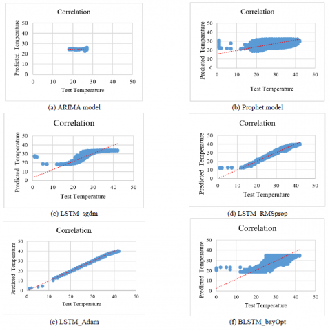
Figure 13 illustrates correlation plots for temperature using six different prediction models. The correlation between the actual test values and the predicted temperature values is depicted in the Figure 13 (a) for the ARIMA model, Figure 13 (b) for the Prophet model, Figure 13 (c) for the LSTM_sgdm model, Figure 13 (d) for LSTM_rmsprop model, Figure 13 (e) for LSTM_adam model, and Figure 13 (f) for BLSTM_bayOpt model. The scatter plot for ARIMA shows no correlation in the prediction of temperature. The scatter plot for Prophet, LSTM_sgdm, LSTM_rmsprop, LSTM_adam, and BLSTM_bayOpt models shows positive correlation in prediction of temperature.
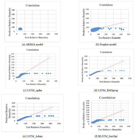
Figure 14 showcases correlation plots demonstrating the relationship between actual test values and predicted temperature values for relative humidity using six distinct prediction models. Each sub-figure corresponds to a specific model: 14 (a) ARIMA, 14 (b) Prophet, 14 (c) LSTM_sgdm, 14 (d) LSTM_rmsprop, 14 (e) LSTM_adam, and 14 (f) BLSTM_bayOpt. The scatter plot for ARIMA shows no correlation in the prediction of relative humidity. The scatter plot for Prophet, LSTM_sgdm, LSTM_rmsprop, LSTM_adam, and BLSTM_bayOpt models shows a positive correlation in the prediction of relative humidity.
Figure 12. Average relative humidity in Pune
Table 2. Proposed work V/s other existing works in prediction work
|
Ref |
Model |
Prediction |
RMSE |
R2 |
|
[39] |
ARIMA |
Financial data |
5.999 |
-- |
|
LSTM |
0.936 |
-- |
||
|
[22] |
LSTM |
Photovoltaic power |
1.195 |
0.837 |
|
BLSTM |
1.135 |
0.879 |
||
|
[1] |
Stepwise regression |
Temperature and relative humidity |
6.129 |
0.832 |
|
[27] |
M1 |
temperature |
8.56 |
0.56 |
|
M2 |
temperature |
9.56 |
0.45 |
|
|
M3 |
Relative humidity |
12.09 |
0.12 |
|
|
[26] |
Prophet |
temperature |
5.7573 |
-- |
|
[23] |
LSTM_adam |
temperature |
1.23 |
-- |
|
LSTM_rmsprop |
1.45 |
-- |
||
|
Prophet |
1.03 |
-- |
||
|
[28] |
Stepwise regression |
Temperature, rainfall, relative humidity and windspeed |
0.58 |
0.82 |
|
Proposed work |
ARIMA |
Temperature |
1.9737 |
-0.004 |
|
Prophet |
4.2417 |
0.2196 |
||
|
LSTM_sgdm |
1.9034 |
0.9948 |
||
|
LSTM_rmsprop |
0.6102 |
0.9830 |
||
|
LSTM_adam |
0.2270 |
0.9976 |
||
|
BLSTM_bayOpt |
1.1573 |
0.9324 |
||
|
ARIMA |
Relative humidity |
6.7238 |
0.7314 |
|
|
Prophet |
21.8952 |
0.4658 |
||
|
LSTM_sgdm |
10.8579 |
0.8260 |
||
|
LSTM_rmsprop |
7.6060 |
0.9146 |
||
|
LSTM_adam |
7.2065 |
0.9233 |
||
|
BLSTM_bayOpt |
5.5509 |
0.9475 |
Table 3. Performance parameters for prediction of temperature and relative humidity
|
Model |
RMSE |
NRMSE |
MAE |
MAPE |
R2 |
Adjusted R2 |
|
Temperature |
||||||
|
ARIMA |
1.9738 |
0.1481 |
1.3667 |
0.0514 |
-0.004 |
-0.0041 |
|
Prophet |
4.2417 |
0.3182 |
3.1504 |
15.7016 |
0.2197 |
0.2196 |
|
LSTM_sgdm |
1.9034 |
0.1428 |
1.4424 |
7.3362 |
0.9948 |
0.9948 |
|
LSTM_rmsprop |
0.6102 |
0.0458 |
0.3673 |
2.1962 |
0.9830 |
0.9830 |
|
LSTM_adam |
0.2270 |
0.0170 |
0.1740 |
0.7840 |
0.9976 |
0.9976 |
|
LSTM_bayOpt |
1.1573 |
0.0868 |
1.4556 |
0.0556 |
0.9324 |
0.93239 |
|
|
Relative Humidity |
|||||
|
ARIMA |
6.7239 |
0.0900 |
5.1714 |
0.1063 |
0.7314 |
0.73138 |
|
Prophet |
21.8952 |
0.29307 |
14.6847 |
38.7652 |
0.4659 |
0.46581 |
|
LSTM_sgdm |
10.8579 |
0.1453 |
5.8540 |
15.1169 |
0.8260 |
0.82596 |
|
LSTM_rmsprop |
7.6060 |
0.1018 |
1.0877 |
2.0360 |
0.9146 |
0.9146 |
|
LSTM_adam |
7.2065 |
0.0965 |
1.0234 |
1.9271 |
0.9233 |
0.92333 |
|
LSTM_bayOpt |
5.5509 |
0.0743 |
1.7013 |
0.0927 |
0.9475 |
0.9475 |
Table 4. ANOVA analysis of performance parameters evaluated for prediction
|
Source of Variation |
SS |
Df |
MS |
F |
P-Value |
F Crit |
Significance |
|
Parameters |
277.7525 |
1 |
277.7525 |
11.0403 |
0.0061 |
4.7472 |
** |
|
Model |
1040.334 |
5 |
208.0668 |
8.2703 |
0.0013 |
3.1058 |
** |
|
parameters X Model |
245.5888 |
5 |
49.1177 |
1.9523 |
0.1588 |
3.1058 |
NS |
|
Within |
301.8968 |
12 |
25.1580 |
|
|||
|
Total |
1865.572 |
23 |
|
*** p<0.001, **p<0.01, *p<0.05; NS, p≥0.05
Statisticians created an analysis of variance (ANOVA) to analyze the results of experimental designs using statistical tests [60]. ANOVA was selected as the preferred statistical method due to its versatility in handling comparisons across multiple groups. It not only identifies significant differences between these groups but also offers insights into the extent or size of these differences. By analyzing the variance between groups in relation to the variance within groups, ANOVA efficiently detects distinctions among multiple sets of data. It is worth noting that ANOVA assumes normal distribution and equal variances within each group, aligning with established statistical assumptions. Additionally, its widespread use and acceptance within the scientific community facilitate clearer communication and interpretation of research findings. The ANOVA analysis is employed to assess the performance metrics of the proposed models, encompassing ARIMA, Prophet, LSTM_sgdm, LSTM_rmsprop, LSTM_adam, and BLSTM_bayOpt in predicting temperature and relative humidity. These results are presented in Tables 4, showcasing parameters such as Sum of Squares (SS), degrees of freedom (df), mean squares (MS), p-value, F value, and F critical value. The p-value, in conjunction with comparison to the F critical value, is utilized to ascertain statistical significance. Notably, a p-value falling between 0.0001 to 0.001 denotes extreme statistical significance, while a range of 0.001 to 0.01 indicates high statistical significance. A p-value within the range of 0.01 to 0.05 signifies statistical significance. In the study by Bhardwaj et al. [27, 61], a finding is considered statistically significant if the p-value is less than or equal to 0.05, and there is no statistical significance when the p-value is greater than 0.05. The p-value is 0.0061 for the performance parameters, and the p-value is 0.0013 for the different models showing statistical significance in the performance parameters and the models.
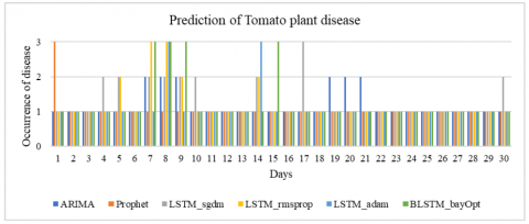
Based on the prediction of temperature and relative humidity with the proposed models, the disease occurrence in the tomato plant is shown in Figure 15. The possible occurrence of disease for 30 days is shown here. The vertical axis shows the category of disease. The number 1 belongs to the healthy class or no disease, the number 2 belongs to early blight, and the number 3 belongs to late blight disease in tomato plants during this period. During this tenure, the most occurring disease in the tomato plant is early blight and late blight. Early blight occurs from 14°C to 38°C and a relative humidity of 54% to 93%. Late blight occurs from 10°C to 22°C and relative humidity of more than 90%. It is seen that around the 7th day, the disease occurs, which is predicted by most of the models. A remedial precaution can be taken on the 6th day by applying the relevant pesticide or herbicide to avoid the occurrence of the disease.
Figure 13. Scatter plot of the True and predicted temperature for the proposed work
Figure 14. Scatter plot of the True and predicted Relative Humidity for the proposed work
Figure 15. Prediction of occurrence of TPD
ARIMA models might struggle to capture complex seasonal patterns in the data, especially when the seasonality is not easily defined or changes over time [62]. The prophet model might not offer the same level of flexibility as more complex models in capturing intricate relationships present in the data [63]. LSTMs can be sensitive to the choice of hyperparameters and may require extensive tuning for optimal performance [64]. The performance of Bayesian optimization models can be sensitive to the choice of hyperparameters [65].
The implications of the above constraints is that there can be a small variation in the accuracy of the data. So future researchers need to keep that tolerance factor in mind regarding accuracy.
Temperature and relative humidity are significant reasons behind the occurrence of disease in plants. Accurate temperature and relative humidity prediction help effectively take a management step toward disease occurrence in tomato plants. The proposed hybrid BLSTM_bayOpt model better predicts the meteorological factors for the Pune region of Maharashtra, India. The RMSE of the proposed model is 1.1573 and 5.5509, MAPE is 0.0556 and 0.0927, R2 is 0.9324 and 0.9475 for temperature and relative humidity, respectively. The proposed model can predict future diseases in plants with a high accuracy rate. The performance parameters show statistical significance with the prediction models. The prediction model can be deployed on a mobile phone to predict the weather parameters in future work. Based on that, the possible occurrence of the disease in the tomato plant can be known to the farmers and stakeholders can in advance, and they can do the management step of applying the required pesticide to reduce the loss in the yield due to disease. Implementing our model in precision agriculture can empower farmers to make informed decisions about irrigation scheduling, disease prevention measures, and crop protection strategies for other crops as well. This integration of advanced predictive models into agricultural systems represents a tangible opportunity to revolutionize traditional farming practices, enabling more efficient resource utilization and sustainable agricultural production. This will involve the potential integration of our model into existing agricultural systems, emphasizing its role in enhancing crop health monitoring, disease prevention, and ultimately improving agricultural productivity.
[1] Gupta, V., Razdan, V.K., Sharma, S., Fatima, K. (2020). Progress and severity of early blight of tomato in relation to weather variables in Jammu province. Journal of Agrometeorology, 22(2): 198-202. https://doi.org/10.54386/jam.v22i2.168
[2] Kim, H.S., Do, K.S., Park, J.H., Kang, W.S., Lee, Y.H., Park, E.W. (2020). Application of numerical weather prediction data to estimate infection risk of bacterial grain rot of rice in Korea. The Plant Pathology Journal, 36(1): 54-66. https://doi.org/10.5423%2FPPJ.OA.11.2019.0281
[3] Ganguli, P., Coulibaly, P. (2019). Assessment of future changes in intensity-duration-frequency curves for southern ontario using North American (NA)-CORDEX models with nonstationary methods. Journal of Hydrology: Regional Studies, 22: 100587. https://doi.org/10.1016/j.ejrh.2018.12.007
[4] Fathi, M., Haghi Kashani, M., Jameii, S.M., Mahdipour, E. (2022). Big data analytics in weather forecasting: A systematic review. Archives of Computational Methods in Engineering, 29(2): 1247-1275. https://doi.org/10.1007/s11831-021-09630-6
[5] Mehrkanoon, S. (2019). Deep shared representation learning for weather elements forecasting. Knowledge-Based Systems, 179: 120-128. https://doi.org/10.1016/j.knosys.2019.05.009
[6] Hossain, M.S., Qian, L., Arshad, M., Shahid, S., Fahad, S., Akhter, J. (2018). Climate change and crop farming in Bangladesh: An analysis of economic impacts. International Journal of Climate Change Strategies and Management, 11(3): 424-440. https://doi.org/10.1108/IJCCSM-04-2018-0030
[7] Bushara, N.O., Abraham, A. (2013). Computational intelligence in weather forecasting: A review. Journal of Network and Innovative Computing, 1(2013): 320-331. https://doi.org/10.1007/s11431-010-4205-z
[8] Torres, J.F., Hadjout, D., Sebaa, A., Martínez-Álvarez, F., Troncoso, A. (2021). Deep learning for time series forecasting: A survey. Big Data, 9(1): 3-21. https://doi.org/10.1089/big.2020.0159
[9] Wang, H., Ma, Z. (2012). Prediction of wheat stripe rust based on neural networks. In Computer and Computing Technologies in Agriculture V: 5th IFIP TC 5/SIG 5.1 Conference, CCTA 2011, Beijing, China, October 29-31, 2011, Proceedings, Part II. Springer Berlin Heidelberg, 5: 504-515. https://doi.org/10.1007/978-3-642-27278-3_52
[10] Zhang, J., Huang, Y., Pu, R., Gonzalez-Moreno, P., Yuan, L., Wu, K., Huang, W. (2019). Monitoring plant diseases and pests through remote sensing technology: A review. Computers and Electronics in Agriculture, 165: 104943. https://doi.org/10.1016/j.compag.2019.104943
[11] Lim, B., Zohren, S. (2021). Time-series forecasting with deep learning: A survey. Philosophical Transactions of the Royal Society A, 379(2194): 20200209. https://doi.org/10.1098/rsta.2020.0209
[12] Xiao, Q., Li, W., Kai, Y., Chen, P., Zhang, J., Wang, B. (2019). Occurrence prediction of pests and diseases in cotton on the basis of weather factors by long short term memory network. BMC Bioinformatics, 20: 1-15. https://doi.org/10.1186/s12859-019-3262-y
[13] Jin, X.B., Wang, H.X., Wang, X.Y., Bai, Y.T., Su, T.L., Kong, J.L. (2020). Deep-learning prediction model with serial two-level decomposition based on bayesian optimization. Complexity, 2020: 1-14. https://doi.org/10.1155/2020/4346803
[14] Khan, F., Kanwal, S., Alamri, S., Mumtaz, B. (2020). Hyper-parameter optimization of classifiers, using an artificial immune network and its application to software bug prediction. IEEE Access, 8: 20954-20964. https://doi.org/10.1109/ACCESS.2020.2968362
[15] Garbelotto, M., Gonthier, P. (2017). Variability and disturbances as key factors in forest pathology and plant health studies. Forests, 8(11): 441. https://doi.org/10.3390/f8110441
[16] Ryalls, J.M., Harrington, R. (2017). Climate and atmospheric change impacts on aphids as vectors of plant diseases. Global Climate Change and Terrestrial Invertebrates, 148-175. https://doi.org/10.1002/9781119070894.ch9
[17] Shivling, V.D., Ghanshyam, C., Kumar, R., Kumar, S., Sharma, R., Kumar, D., Sharma, A., Sharma, S.K. (2017). Prediction model for predicting powdery mildew using ANN for medicinal plant-picrorhiza kurrooa. Journal of The Institution of Engineers (India): Series B, 98: 77-81. https://doi.org/10.1007/s40031-016-0225-9
[18] Deb, S., Bharpoda, T.M. (2017). Impact of meteorological factors on population of major insect pests in tomato, Lycopersicon esculentum Mill. under middle gujarat condition. Journal of Agrometeorology, 19(3): 251-254. https://doi.org/10.54386/jam.v19i3.665
[19] Munir, M. (2018). Plant disease epidemiology: Disease triangle and forecasting mechanisms in highlights. Hosts Virus, 5(1): 7-11. https://doi.org/10.17582/journal.hv/2018/5.1.7.11
[20] Shah, D.A., Paul, P.A., De Wolf, E.D., Madden, L.V. (2019). Predicting plant disease epidemics from functionally represented weather series. Philosophical Transactions of the Royal Society B, 374(1775): 20180273. https://doi.org/10.1098/rstb.2018.0273
[21] Chhetri, M., Kumar, S., Pratim Roy, P., Kim, B.G. (2020). Deep BLSTM-GRU model for monthly rainfall prediction: A case study of Simtokha, Bhutan. Remote Sensing, 12(19): 3174. https://doi.org/10.3390/rs12193174
[22] Yang, T., Li, B., Xun, Q. (2019). LSTM-attention-embedding model-based day-ahead prediction of photovoltaic power output using Bayesian optimization. IEEE Access, 7: 171471-171484. https://doi.org/10.1109/ACCESS.2019.2954290
[23] Toharudin, T., Pontoh, R.S., Caraka, R.E., Zahroh, S., Lee, Y., Chen, R.C. (2023). Employing long short-term memory and facebook prophet model in air temperature forecasting. Communications in Statistics-Simulation and Computation, 52(2): 279-290. https://doi.org/10.1080/03610918.2020.1854302
[24] Xu, W., Wang, Q., Chen, R. (2018). Spatio-temporal prediction of crop disease severity for agricultural emergency management based on recurrent neural networks. GeoInformatica, 22: 363-381. https://doi.org/10.1007/s10707-017-0314-1
[25] Wang, H., Sanchez-Molina, J.A., Li, M., Rodríguez Díaz, F. (2019). Improving the performance of vegetable leaf wetness duration models in greenhouses using decision tree learning. Water, 11(1): 158. https://doi.org/10.3390/w11010158
[26] Oo, Z.Z., Sabai, P.H.Y.U. (2020). Time series prediction based on facebook prophet: A case study, temperature forecasting in Myintkyina. International Journal of Applied Mathematics Electronics and Computers, 8(4): 263-267. https://doi.org/10.18100/ijamec.816894
[27] Bhardwaj, N.R., Atri, A., Rani, U., Banyal, D.K., Roy, A.K. (2021). Weather-based models for predicting risk of zonate leaf spot disease in Sorghum. Tropical Plant Pathology, 46: 702-713. https://doi.org/10.1007/s40858-021-00461-1
[28] Dar, W.A., Parry, F.A., Bhat, B.A. (2021). Potato late blight disease prediction using meteorological parameters in Northern Himalayas of India. Journal of Agrometeorology, 23(3): 310-315. https://doi.org/10.54386/jam.v23i3.35
[29] Taylor, S.J., Letham, B. (2018). Forecasting at scale. The American Statistician, 72(1): 37-45. https://doi.org/10.1080/00031305.2017.1380080
[30] Soneji, H. (2020). Historical Weather Data for Indian Cities. https://www.kaggle.com/hiteshsoneji/historical-weather-data-for-indian-cities, accessed on Jan. 15, 2021.
[31] Lawrence, M.G. (2005). The relationship between relative humidity and the dewpoint temperature in moist air: A simple conversion and applications. Bulletin of the American Meteorological Society, 86(2): 225-234. https://doi.org/10.1175/BAMS-86-2-225
[32] Ghiasi, R., Ghasemi, M.R., Noori, M. (2018). Comparative studies of metamodeling and AI-Based techniques in damage detection of structures. Advances in Engineering Software, 125: 101-112. https://doi.org/10.1016/j.advengsoft.2018.02.006
[33] Wang, Y., Xu, C., Zhang, S., Yang, L., Wang, Z., Zhu, Y., Yuan, J. (2019). Development and evaluation of a deep learning approach for modeling seasonality and trends in hand-foot-mouth disease incidence in mainland China. Scientific Reports, 9(1): 8046. https://doi.org/10.1038/s41598-019-44469-9
[34] Feng, M., Zheng, J., Ren, J., Hussain, A., Li, X., Xi, Y., Liu, Q. (2019). Big data analytics and mining for effective visualization and trends forecasting of crime data. IEEE Access, 7: 106111-106123. https://doi.org/10.1109/ACCESS.2019.2930410
[35] Lai, G., Chang, W.C., Yang, Y., Liu, H. (2018). Modeling long-and short-term temporal patterns with deep neural networks. In The 41st International ACM SIGIR Conference On Research & Development In Information Retrieval, pp. 95-104. https://doi.org/10.1145/3209978.3210006
[36] Zhang, Q., Hu, W., Liu, Z., Tan, J. (2020). TBM performance prediction with Bayesian optimization and automated machine learning. Tunnelling and Underground Space Technology, 103: 103493. https://doi.org/10.1016/j.tust.2020.103493
[37] Abebe, T.H. (2020). Time series analysis of monthly average temperature and rainfall using seasonal ARIMA model (in Case of Ambo Area, Ethiopia). International Journal of Theoretical and Applied Mathematics, 6(5): 76-87. https://doi.org/10.11648/j.ijtam.20200605.13
[38] Youssef, J., Ishker, N., Fakhreddine, N. (2021). Economic forecast of the wealthiest gulf countries using ARIMA model. Journal of Applied Economic Sciences, 16(2): 228-237.
[39] Siami-Namini, S., Tavakoli, N., Namin, A.S. (2018). A comparison of ARIMA and LSTM in forecasting time series. In 2018 17th IEEE International Conference on Machine Learning and Applications (ICMLA), Orlando, FL, USA, pp. 1394-1401. https://doi.org/10.1109/ICMLA.2018.00227
[40] Kumar, R.R., Baishya, M. (2020). Forecasting of Potato prices in India: An application of Arima model. Economic Affairs, 65(4): 473-479. https://doi.org/10.46852/0424-2513.4.2020.1
[41] Duarte, D., Faerman, J. (2019). Comparison of time series prediction of healthcare emergency department indicators with ARIMA and Prophet. In Computer Science & Information Technology (CS & IT) Computer Science Conference, pp. 123-133. https://doi.org/10.5121/csit.2019.91810
[42] Hochreiter, S. Schmidhuber, J. (1997). Long short-term memory. Neural Comput, 9(8): 1-32. https://doi.org/ 10.1162/neco.1997.9.8.1735
[43] Li, H., Zhu, L., Gong, H., Sun, H., Yu, J. (2020). Land subsidence modelling using a long short-term memory algorithm based on time-series datasets. Proceedings of the International Association of Hydrological Sciences, 382: 505-510. https://doi.org/10.5194/piahs-382-505-2020
[44] Qian, L., Hu, L., Zhao, L., Wang, T., Jiang, R. (2020). Sequence-dropout block for reducing overfitting problem in image classification. IEEE Access, 8: 62830-62840. https://doi.org/10.1109/ACCESS.2020.2983774
[45] Graves, A., Schmidhuber, J. (2005). Framewise phoneme classification with bidirectional LSTM and other neural network architectures. Neural Networks, 18(5-6): 602-610. https://doi.org/10.1016/j.neunet.2005.06.042
[46] Radman, A., Suandi, S.A. (2021). BiLSTM regression model for face sketch synthesis using sequential patterns. Neural Computing and Applications, 33: 12689-12702. https://doi.org/10.1007/s00521-021-05916-9
[47] Kim, C., Fuxin, L., Alotaibi, M., Rehg, J.M. (2021). Discriminative appearance modeling with multi-track pooling for real-time multi-object tracking. In Proceedings of the IEEE/CVF Conference on Computer Vision and Pattern Recognition, Nashville, TN, USA, pp. 9553-9562. https://doi.org/10.1109/CVPR46437.2021.00943
[48] Victoria, A.H., Maragatham, G. (2021). Automatic tuning of hyperparameters using Bayesian optimization. Evolving Systems, 12: 217-223. https://doi.org/10.1007/s12530-020-09345-2
[49] He, F., Zhou, J., Feng, Z.K., Liu, G., Yang, Y. (2019). A hybrid short-term load forecasting model based on variational mode decomposition and long short-term memory networks considering relevant factors with Bayesian optimization algorithm. Applied Energy, 237: 103-116. https://doi.org/10.1016/j.apenergy.2019.01.055
[50] Chothani, E.P., Kapadiya, H.J., Acharya, M.F., Bhaliya, C.M. (2017). Impact of weather parameter on early blight epidemiology in tomato crop. International Journal of Current Microbiology and Applied Sciences, 6(11): 3160-3166. https://doi.org/10.20546/ijcmas.2017.611.370
[51] Singh, V.K., Shailbala, P.V. (2012). Forecasting models: An effective toos for potato late blight management. Eco-friendly Innovative Approaches in Plant Disease Management. International Book Distributors and Publisher, New Delhi, 102-112. https://doi.org/10.13140/RG.2.1.1856.9369
[52] Schumann, G.L., D’Arcy, C.J. (2021). Late blight of potato and tomato. University of Minnesota Extension. https://www.apsnet.org/edcenter/disandpath/oomycete/p https://doi.org/10.1094/PHI-I-2000-0724-01
[53] Shternshis, M., Asaturova, A., Shpatova, T., Zhevnova, N., Homyak, A. (2021). Promising Bacillus subtilis strains BZR 336g and BZR 517 for biocontrol of blackcurrant against Septoria leaf spot under unfavorable climate conditions. Journal of Plant Pathology, 103(1): 295-298. https://doi.org/10.1007/s42161-020-00660-w
[54] Kamei, A., Dutta, S., Sarker, K., Das, S., Datta, G., Goldar, S. (2018). Target leaf spot of tomato incited by Corynespora cassiicola, an emerging disease in tomato production under Gangetic alluvial region of West Bengal, India. Archives of Phytopathology and Plant Protection, 51(19-20): 1039-1048. https://doi.org/10.1080/03235408.2018.1545281
[55] Wagle, S.A., Harikrishnan, R. (2022). Prediction of tomato plant disease with meteorological condition and artificial intelligence. ECS Transactions, 107(1): 20377. https://doi.org/10.1149/10701.20377ecst
[56] Araújo, E.R., Pereira, R.C., Ferreira, M.A.S.V., Café-Filho, A.C., Moita, A.W., Quezado-Duval, A.M. (2010). Effect of temperature on pathogenicity components of tomato bacterial spot and competition between Xanthomonas perforans and X. gardneri. In III International Symposium on Tomato Diseases, 914: 39-42. https://doi.org/10.17660/ActaHortic.2011.914.3
[57] Imran, M., Khan, M.A., Fiaz, M., Azeem, M., Mustafa, M. (2013). Influence of environmental conditions on tomato mosaic virus disease development under natural condition. Pakistan Journal of Phytopathology, 25(2): 117-122.
[58] Hossain, M., Akanda, A., Hossain, M. (2010). Environmental effect on toma toyellow leaf curl virus and whitefly population in tomato varieties under field condition. Annals of Bangladesh Agriculture, 14(1-2): 1-8.
[59] Pick, J.L., Nakagawa, S., Noble, D.W. (2019). Reproducible, flexible and high‐throughput data extraction from primary literature: The metaDigitise r package. Methods in Ecology and Evolution, 10(3): 426-431. https://doi.org/10.1111/2041-210X.13118
[60] De Agustina, B., Rubio, E.M., Sebastián, M.Á. (2014). Surface roughness model based on force sensors for the prediction of the tool wear. Sensors, 14(4): 6393-6408. https://doi.org/10.3390/s140406393
[61] Honěk, A., Martinková, Z., Brabec, M., Saska, P. (2019). Predicting aphid abundance on winter wheat using suction trap catches. Plant Protection Science, 56(1): 35-45. https://doi.org/10.17221/53/2019-PPS
[62] Hansen, J.V., Nelson, R.D. (1997). Neural networks and traditional time series methods: A synergistic combination in state economic forecasts. IEEE transactions on Neural Networks, 8(4): 863-873. https://doi.org/10.1109/72.595884
[63] Guo, L., Fang, W., Zhao, Q., Wang, X. (2021). The hybrid PROPHET-SVR approach for forecasting product time series demand with seasonality. Computers & Industrial Engineering, 161: 107598. https://doi.org/10.1016/j.cie.2021.107598
[64] Li, W., Ng, W.W., Wang, T., Pelillo, M., Kwong, S. (2021). HELP: An LSTM-based approach to hyperparameter exploration in neural network learning. Neurocomputing, 442: 161-172. https://doi.org/10.1016/j.neucom.2020.12.133
[65] Cho, H., Kim, Y., Lee, E., Choi, D., Lee, Y., Rhee, W. (2020). Basic enhancement strategies when using Bayesian optimization for hyperparameter tuning of deep neural networks. IEEE Access, 8: 52588-52608. https://doi.org/10.1109/ACCESS.2020.2981072