Aymen Takie Eddine Selmi*![]() | Mohamed Faouzi Zerarka
| Mohamed Faouzi Zerarka![]() | Abdelhakim Cheriet
| Abdelhakim Cheriet![]()
© 2024 The authors. This article is published by IIETA and is licensed under the CC BY 4.0 license (http://creativecommons.org/licenses/by/4.0/).
OPEN ACCESS
Traditional K-means clustering may converge to suboptimal solutions due to local optima, impacting cluster balance and compactness. To fix this, we suggest an enhanced K-means algorithm that includes a new step for redistribution post-clustering that is based on the sum of squares errors (SSE) and diameter. Our approach introduces a redistribution step focusing on achieving balanced population distribution within clusters. Evaluation metrics include Davies-Bouldin Index (DBI) and Gini coefficient, quantifying improvements in cluster compactness and balance. We compare our method against traditional K-means on diverse datasets, such that a lower value indicates better clustering results. The post-clustering redistribution significantly reduces DBI and Gini coefficient, indicating enhanced cluster quality and balance. This improvement is consistent across various datasets, showcasing the method's reliability and generalizability. Our improved K-means algorithm achieves better cluster balance and compactness by redistributing post-clustering, which also reduces problems with local optima. The method's applicability extends to diverse domains, providing more reliable clustering outcomes with practical implications in areas such as customer segmentation, anomaly detection, pattern recognition, and resource optimization.
K-means, enhanced K-means, post-clustering redistribution, Davies-Bouldin Index, Gini coefficient
Clustering is a widely used unsupervised learning technique applied across many domains, including market segmentation [1], scientific discovery [2], and recommendation systems [3]. K-means is widely favored as a clustering algorithm due to its simplicity and efficiency [4]. However, K-means can get stuck in a local optimum, where it converges to a suboptimal solution. The algorithm tries to reduce the sum of squared distances between clusters as much as possible (inertia or SSE), but it can hit local optima, which can lead to cluster assignments that aren't the best overall solution. This characteristic should be considered when employing K-means for clustering tasks. To overcome this limitation, several techniques and variations of K-means have been proposed. Researchers often employ two categorical approaches in clustering analysis: Determining the optimal number of clusters (k) is crucial for capturing the inherent structure of the data [5]. Getting a balanced population distribution within clusters improves robustness by lowering the effect of noise and outliers, which leads to more reliable clustering results [6]. Balancing representation improves cluster quality by addressing biases in imbalanced datasets, ensuring fair representation of all clusters, and preventing underrepresented minorities [7]. This population equilibrium not only enhances robustness, but it also makes clustering algorithms better at generalization [6, 7]. This means that the results can be used in real-world situations beyond the training dataset. For example, in customer segmentation, a few dominant customer segments may emerge while others remain underrepresented. In network analysis, a handful of highly connected nodes can skew the population distribution across clusters. Such imbalances pose challenges when analyzing relative cluster importance and prevalence. They can also obscure useful patterns within underpopulated groups.
In this context, inter-dependence and intra-dependence aim to balance compactness within clusters and separation between clusters while achieving a balanced population distribution within clusters [8]. The inter-dependence approach maximizes cluster separation using metrics like the silhouette score [9] and the Davies-Bouldin index [10]. The intra-dependence approach ensures internal cohesion, minimizing intra-cluster variance. Regardless of the approach, a balanced population distribution within clusters is essential to prevent biased results. The Gini coefficient [11] is a valuable metric for achieving this balance.
Extensive research in literature has focused on these key issues: determining the optimal number of clusters (k) and achieving a balanced population distribution within clusters. Common K selection approaches include Elbow method [12] and Silhouette analysis [9], widely applied in real-world contexts such as target identification, school data clustering, opinion mining, poverty grouping, and cloud workload modeling [13-21]. Information Criteria, such as the Bayesian Information Criterion (BIC) [22] or Akaike Information Criterion (AIC) [23] as Stability-based methods like DStab have also been proposed [24, 25]. Additionally, methods like Weighted K-means [26], Oversampling and under-sampling [27, 28], post-clustering redistribution [29, 30] address imbalanced clusters across domains like wind engineering, agricultural grading, and social network analysis [24, 25, 31-35]. Further advancements include efficiency improvements to K-means using evolutionary computation, statistical inference methods for significant cluster selection, and fast clustering algorithms for image quantization [36-38]. However, existing techniques often optimize objectives independently without holistically addressing both.
Given the existence of numerous good ideas aimed at enhancing the clustering quality of the K-means algorithm, we propose an enhanced version of the K-means clustering algorithm by introducing a novel post-processing redistribution step. This step is designed to address the issue of cluster imbalance and improve the overall quality and compactness of the clusters. By adding the postprocessing redistribution technique-based diameter, we were able to greatly lower the evaluation metrics that were used to judge the performance of clustering. This enhancement significantly impacted the balance within the clusters, leading to more well-organized and tightly grouped data points within each cluster.
The following sections of this paper are structured in the following manner. In the present paper, Section 2 provides an overview of the preliminary concepts and background information relevant to our study. Section 3 presents a detailed analysis of the algorithm that we have developed for our research. The experimental results and discussion findings have been succinctly outlined in Sections 4, and 5, while a brief conclusion has been presented in Section 6.
2.1 K-means algorithm
K-means algorithm begins by randomly selecting K centers. To calculate the distance between a sample xj and a center ci, the Euclidean distance formula is used:
$\operatorname{dist}(i, j)=\sum_k^d\left(x_{j k}-c_{i k}\right)^2$ (1)
Here, d represents the dimensionality of the samples. Next, each sample is assigned to the cluster center that is closest to it. In the subsequent step, the cluster centers are updated using the mean of the samples assigned to each cluster:
$c_i^{\prime}=\frac{1}{m_i} \sum_{x_j \in \text { cluster } c_j} x_j$ (2)
where, mi represents the total number of samples belonging to the cluster determined by the center ci. The distances between the samples and cluster centers are recalculated, and this process is repeated until the algorithm converges.
2.2 The Davies-Bouldin Index (DBI)
The Davies-Bouldin Index (DBI) is a measure used to evaluate the quality of clustering results. It quantifies the average similarity between clusters, taking into account both the inter-cluster and intra-cluster distances. A lower DBI value indicates better clustering results.
The formula for calculating the Davies-Bouldin Index for a set of clusters is as follows:
$D B I=\frac{1}{K} \sum_{i=1}^k \max _i\left(\frac{s s w_i+s s w_j}{S S B}\right)$ (3)
DBI is the Davies-Bouldin Index.
K is the total number of clusters.
SSW (Sum of Squares Within a cluster) is a cohesion metric in an i-cluster.
SSB (Sum of Squares Between clusters) is a metric for separating between two clusters.
2.3 The Gini coefficient
The Gini coefficient is a statistical measure that is used to represent the level of income or wealth inequality within a population. It was developed by Italian statistician Corrado Gini in 1912. The coefficient ranges between 0 and 1, where 0 represents perfect equality (everyone has the same income or wealth) and 1 represents perfect inequality (one individual or household possesses all the income or wealth, while others have none).
Mathematically, the Gini coefficient can be expressed as:
$G=(A /(A+B))$ (4)
where: A is the area between the Lorenz curve (a graphical representation of income distribution) and the line of perfect equality.
B is the area under the line of perfect equality.
Given the abundance of promising approaches for addressing the challenge of escaping local optima, our paper introduces an enhanced K-means algorithm that incorporates a post-clustering redistribution technique. The contribution of our work lies in proposing this redistribution method as a means to tackle the problem effectively.
The process of the proposed algorithm shown in Figure 1 is a modified version of the K-means algorithm with iterative refinement. The standard K-means algorithm is an iterative clustering algorithm that aims to partition a given dataset into K clusters, where each data point belongs to the cluster with the nearest mean.
In the process of enhanced K-means, we begin with an initial value of K and then apply the standard k-means algorithm with K clusters on the given dataset. After this initial step, we have two variants to refine the cluster formation.
In the first variant, SSE-Based Cluster Splitting denoted SSE-SPLITTING_KMEANS, we calculate the SSE (sum of squared errors) for each cluster. This helps us identify the cluster with the highest SSE. We then take nci − nci/r points closest to the center of this cluster ci, and these points will define the first cluster. The remaining points are considered residual points.
$S S E=\sum_i^n\left(x_i-\bar{x}\right)^2$ (5)
where, xi denotes each individual data point. $\bar{x}$ represents the mean (average) of all the data points.
Figure 1. The process of the proposed algorithm: Variant 1 (SSE-SPLITTING_KMEANS), Variant 2 (DIAMETER_KMEANS)
For the second variant, Iterative Diameter-Based K-Means denoted DIAMETER_KMEANS, we focus on the diameter of each cluster. Within each cluster, we sort the points based on their distance from the center, starting from the nearest point to the farthest one. Next, we take nci − nci/r nearest points to the center and calculate the new center of each cluster ci based on these selected points. Subsequently, we take residual points, and we determine the point that has the maximum distance to the new center for each cluster. The cluster that minimizes the distances between these maximum distances is then selected as the target cluster. We repeat the same operation as in the first variant for this selected cluster.
The next step involves merging the residual points from the selected cluster with the other clusters. This merging of residual points with other clusters involves a comprehensive criterion for optimizing SSE and diameter, in other term, each residual point is strategically assigned to the cluster that minimizes the increase in SSE and diameter. The algorithm aims to refine the cluster structure, strategically integrating residual points into clusters that exhibit both enhanced compactness and well-managed spatial spread. As a result, we reduce the number of clusters by setting K = K - 1. We then apply the K-means algorithm again, this time on the combined points from the residual clusters and merged points (residual points) with the updated value of K.
We continue iterating through the previous steps until K becomes 0, meaning all clusters have been merged. This iterative process leads to a more refined and optimized clustering solution for the given dataset.
The algorithm aims to enhance the overall clustering quality by merging the data points that exhibit the highest distance within a cluster. The choice of r value can significantly impact the clustering results.
In the rest of this section, we focus on the reasons for using SSE and Diameter for redistribution. On the other hand, we discuss the metrics used to evaluate these proposed enhancements and analyze the complexity of enhanced K-means algorithm.
3.1 Rationale for SSE and diameter criteria in redistribution
The utilization of SSE (Sum of Squared Errors) and diameter as criteria for redistribution in clustering algorithms is rooted in their distinct advantages and complementary roles in evaluating cluster quality. SSE, by measuring the compactness of clusters, encourages the formation of tightly-knit groups, ensuring that data points are closely associated with their respective centroids. This metric offers an intuitive and straightforward interpretation, making it a valuable criterion for assessing intra-cluster cohesion. On the other hand, Diameter, as a redistribution criterion in clustering algorithms, assesses the spatial spread within clusters. It represents the maximum distance between data points, offering insights into overall dispersion. This metric is particularly valuable for accommodating irregular cluster shapes and contributes to creating well-rounded, spatially balanced clusters.
3.2 Proposed enhancement evaluation
The evaluation of these algorithmic variants relies on two key metrics, namely the Davies-Bouldin Index (DBI) and the Gini coefficient. The following points offer a comprehensive rationale for the selection of these metrics, providing a nuanced understanding of the reasons behind their choice in the evaluation of the proposed algorithmic variants.
Why DBI? We chose the DBI as the clustering metric due to its superior performance in both K-means and Bissecting K-means algorithms when compared to external validation metrics. External indexes require prior knowledge, which is often not available in real applications, making them unsuitable for determining the number of clusters. On the other hand, DBI is an internal validation metric that does not rely on prior knowledge and has shown good discrimination ability [39].
In the work [40] that aims to compare various internal validation metrics [40], DBI ranked second overall, just behind another metric called SDbw [41], but DBI was more suitable for real-world applications and showed better performance with more than two clusters. Other internal metrics, like Dunn Index [42], were less effective due to their sensitivity to boundary points. Additionally, in a comprehensive comparison of 30 cluster validity indices, DBI belonged to the group of better performing indices, while some others, like the Dunn Index, did not yield statistically significant results.
Why Gini? The Gini coefficient is frequently chosen as a clustering evaluation metric in various fields due to its ability to quantify inequality or diversity within a set of values [11]. When applied to clustering, the Gini coefficient measures clustering quality and the homogeneity of clusters [43]. Its sensitivity to cluster compactness makes it valuable in assessing the balance and tightness of data points within clusters [43]. Moreover, its adaptability to clusters of arbitrary shapes and sizes makes it versatile for analyzing clustering results with diverse data distributions. The Gini coefficient’s single scalar output ensures easy interpretability and facilitates comparisons across different clustering experiments [11].
Therefore, the measurements we have chosen are based on the goal of thoroughly evaluating the proposed enhancements. DBI is employed to measure the compactness of clusters, providing insights into the intra-cluster similarity and separation between clusters. Meanwhile, the Gini coefficient is utilized to quantify the balance within clusters, offering a robust measure of population distribution.
3.3 The complexity of enhanced K-means algorithm
Analyzing the time complexity of enhanced K-means algorithm involves a detailed examination of the computational costs associated with each step. In the standard K-means initialization, the complexity is expressed as O(n.K.d.I). Where n is the number of data points, K is the initial number of clusters, d is the dimensionality of the data, and I is the number of iterations until convergence.
For the SSE-Based Cluster Splitting variant (SSE-SPLITTING_KMEANS), an additional computational complexity of O(n.K.I) is introduced. This involves calculating the sum of squared errors (SSE) for each cluster and selecting points based on SSE. The Iterative Diameter-Based K-Means variant (DIAMETER_KMEANS) introduces a complexity of O(n.K. log(n).I) as it entails sorting points based on their distances within each cluster.
Merging residual clusters contributes O(n.I) to the computational complexity, involving the merging of points and updating the number of clusters. Considering the overall iterative process, denoted by T as the number of iterations until K becomes 0. The total computational complexity is expressed as O(T.(n.K.d.I+n.K.I+n.I)) for SSE-SPLITTING_KMEANS; O(T.(n.K.d.I+n.K.log(n).I+n.I)) for DIAMETER_KMEANS. This comprehensive evaluation captures the complexity associated with each phase of enhanced K-means algorithm, providing insights into its computational efficiency and performance characteristics.
4.1 Experimental environment
For the implementation of our proposition, we utilize a 5-core CPU PC running a 64-bit Mac OS operating system, with 8GB of memory and a 128GB SSD. To support our algorithm, we employ Anaconda, an open-source platform for Python data science. Furthermore, we adapt and utilize the K-means implementation in Scikit-learn, a Python-based, free, and efficient machine learning tool, for our experiments.
4.2 Selection of TSP benchmark for evaluation
To validate our proposal, we chose a dataset used in the well-known TSP (Traveling Salesman Problem) [44]. The use of TSP optimization benchmarks as a dataset when the machine learning techniques are used is one of the main focuses of optimization community [45-47]. The use of clustering as a step in the optimization techniques was introduced in many works such as [48-52].
The instances used refer to specific problems in the Traveling Salesman Problem (TSP) where the cities are represented as points in an Euclidean space. In these instances, the cities are typically defined by their (x, y) coordinates in a two-dimensional plane, and the distance between two cities is calculated using the Euclidean distance [53].
We assess the performance of our clustering algorithm on five different datasets: Berlin52, eil51, eil76, kroA100, and eil101. These datasets are selected from the TSPLIB [44] library and represent sample instances for the Traveling Salesman Problem (TSP). All of these datasets will be utilized for clustering, and we will conduct evaluations on each of them using various metrics.
Given that the dataset instances lie in a two-dimensional plane, we aim to employ a quadtree structure to represent these instances. Our focus is on utilizing the quadtree representation for the proposed enhancement of the k-means clustering approach with a targeted range of 3 to 4 clusters.
The evaluation of the proposed algorithm and its two variants involves applying it to five distinct instances. Additionally, a comparison is made between the performance of enhanced K-means and the standard K-means. The evaluation metrics used are the Davies-Bouldin Index (DBI) to assess clustering quality and cluster compactness and the Gini coefficient to measure the distribution of results among the clusters. The value of r in our proposition plays a vital role as a key parameter that directly impacts both the quality of clustering and the distribution of points across the clusters.
The comparative analysis of clustering techniques presented in Table 1, including standard K-means and enhanced K-means variants (1 and 2), was conducted on multiple instances of the TSP. The results indicate that enhanced variants consistently outperformed standard K-means in terms of the DBI metric, with DIAMETER_KMEANS achieving the best cluster separation and compactness. While Gini values were similar across all methods, enhanced variants showed potential for a more balanced data distribution among clusters. In conclusion, enhanced K-means variants, particularly DIAMETER_KMEANS, demonstrate higher clustering quality, compactness, and potentially achieve a more balanced distribution of data points among clusters compared to the standard K-means algorithm.
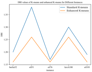
Focusing solely on DBI values, the results suggest that both our enhanced K-means variants (1 and 2) perform slightly better than the standard K-means algorithm in terms of clustering quality and cluster compactness. DIAMETER_KMEANS consistently achieves the best results in terms of DBI (Table 2). For instance, in Eil51, DIAMETER_KMEANS achieves the lowest DBI of 1.16 compared to 1.20 for K-means and 1.17 for SSE-SPLITTING_KMEANS. Similar trends are observed in Berlin52, Eil76, KroA100, instances, where DIAMETER_KMEANS consistently yields the lowest DBI values, emphasizing its superior performance in clustering. See Figure 2.
As measured by the Gini values, the results show that both SSE-SPLITTING_KMEANS and DIAMETER_KMEANS achieve a slightly more balanced distribution of data points among clusters than the standard K-means. When looking at Gini, the optimal results are consistently obtained with DIAMETER_KMEANS (Table 3). For instances (e.g., KroA100, Eil76, and Eil101), DIAMETER_KMEANS achieves the lowest Gini, respectively, 0.26, 0.22, and 2.21; and seems to outperform both KMEANS and SSE-SPLITTING_KMEANS. KroA100 has higher Gini indices across all methods, indicating that clustering performance might be more challenging for this instance. See Figure 3.
Our comprehensive experimental investigations illuminate how two pivotal parameters, denoted as r1 and r2, influence the optimization efficacy of the proposed enhanced K-means variants across diverse problem instances. Fixing K at 3 clusters, we meticulously explore the impact of varying r1 and r2 values on the performance of SSE-SPLITTING_KMEANS and DIAMETER_KMEANS based on key evaluation metrics. The ideal parameter settings are contingent on the prevailing optimization objectives, as encapsulated in Table 4.
Table 1. DBI and Gini values for different instances and methods in K-means and enhanced K-means variants
|
Instance |
Method |
DBI |
Gini |
|
Eil51 |
K-means SSE-SPLITTING_KMEANS DIAMETER_KMEANS |
1.20 1.19 1.17 |
0.23 0.21 0.22 |
|
Berlin52 |
K-means SSE-SPLITTING_KMEANS DIAMETER_KMEANS |
1.38 1.27 1.36 |
0.26 0.23 0.24 |
|
Eil76 |
K-means SSE-SPLITTING_KMEANS DIAMETER_KMEANS |
1.17 1.16 1.16 |
0.24 0.23 0.24 |
|
KroA100 |
K-means SSE-SPLITTING_KMEANS DIAMETER_KMEANS |
1.30 1.30 1.26 |
0.30 0.26 0.29 |
|
Eil101 |
K-means SSE-SPLITTING_KMEANS DIAMETER_KMEANS |
1.19 1.18 1.17 |
0.24 0.23 0.24 |
Table 2. DBI values of K-means and enhanced K-means variants for different instances
|
Instance |
Method |
DBI |
|
Eil51 |
K-means SSE-SPLITTING_KMEANS DIAMETER_KMEANS |
1.20 1.17 1.16 |
|
Berlin52
|
K-means SSE-SPLITTING_KMEANS DIAMETER_KMEANS |
1.38 1.26 1.35 |
|
Eil76 |
K-means SSE-SPLITTING_KMEANS DIAMETER_KMEANS |
1.17 1.16 1.16 |
|
KroA100 |
K-means SSE-SPLITTING_KMEANS DIAMETER_KMEANS |
1.30 1.29 1.26 |
|
Eil101 |
K-means SSE-SPLITTING_KMEANS DIAMETER_KM EANS |
1.19 1.16 1.17 |
Figure 2. Ilustration of DBI values of K-means and enhanced K-means for different instances
Table 3. Gini values of K-means and enhanced K-means variants for different instances
|
Instance |
Method |
Gini |
|
Eil51 |
K-means SSE-SPLITTING_KMEANS DIAMETER_KMEANS |
0.23 0.18 0.20 |
|
Berlin52 |
K-means SSE-SPLITTING_KMEANS DIAMETER_KMEANS |
0.26 0.21 0.23 |
|
Eil76 |
K-means SSE-SPLITTING_KMEANS DIAMETER_KMEANS |
0.24 0.23 0.22 |
|
KroA100 |
K-means SSE-SPLITTING_KMEANS DIAMETER_KMEANS |
0.30 0.26 0.26 |
|
Eil101 |
K-means SSE-SPLITTING_KMEANS DIAMETER_KMEANS |
0.24 0.22 0.21 |
Table 4. Ideal r values to optimize performance of enhanced K-means variants for different instances
|
Instance |
Method |
Metric |
r1 |
r2 |
|
Eil51 |
SSE-SPLITTING_KMEANS DIAMETER_KMEANS |
DBI Gini DBI+Gini DBI Gini DBI+Gini |
6 2 5 5.25 6 5 |
2.5 1.75 2 2.25 2 2 |
|
Berlin52 |
SSE-SPLITTING_KMEANS DIAMETER_KMEANS |
DBI Gini DBI+Gini DBI Gini DBI+Gini |
8 4 4 3 4 3 |
4 1.5 4 1.5 1.5 1.75 |
|
Eil76 |
SSE-SPLITTING_KMEANS DIAMETER_KMEANS |
DBI Gini DBI+Gini DBI Gini DBI+Gini |
1.75 1.75 1.75 3.5 4 3.5 |
3 3 3 6 1.5 6 |
|
KroA100 |
SSE-SPLITTING_KMEANS DIAMETER_KMEANS |
DBI Gini DBI+Gini DBI Gini DBI+Gini |
2.75 3 3 1.5 1.25 1.5 |
1.75 1.5 1.5 4 4 4 |
|
Eil101 |
SSE-SPLITTING_KMEANS DIAMETER_KMEANS |
DBI Gini DBI+Gini DBI Gini DBI+Gini |
1.75 1.75 1.75 2.5 2.5 2.5 |
5 1.75 3 3.5 1.25 3.5 |
When maximizing cluster separation and compactness per the DBI, optimal r1and r2 values for DIAMETER_KMEANS hover between 3.5-6, while SSE-SPLITTING_KMEANS thrives at approximately 1.5-8. These carefully selected parameters allow our enhanced K-means variants to cultivate distinct, tightly-knit clusters, overcoming the limitations of conventional K-means. Conversely, if crafting clusters with balanced data distributions is paramount measured through the Gini coefficient, both variants flourish when r1 and r2 are tuned between 1.25-4. This parametrization empowers the creation of equitably populated clusters, surmounting imbalances. Considering the composite metric amalgamating Gini and DBI, our variants demonstrate resilient performance across diverse instances. For situations where DBI reductions through improved cluster cohesion take precedence, optimal r1 and r2 values for DIAMETER_KMEANS and SSE-SPLITTING_KMEANS situate around 3.5-6 and 1.5-8 respectively. In summary, our exhaustive experiments elucidate the profound influence of r1 and r2 on the optimization capabilities of our enhanced K-means variants, providing insights into ideal parameter ranges based on specified optimization objectives.
Figure 3. Ilustration of Gini values of K-means and enhanced K-means for different instances
In this study, we proposed an enhanced K-means clustering algorithm with a post-processing step to achieve balanced cluster sizes. Our algorithm uses SSE and a diameter-based criterion during redistribution of points between clusters. The key findings of our experiments are:
(1) Our enhanced algorithm resulted in an average of 2.6-4% reduction in Davies-Bouldin Index compared to standard K-means, demonstrating improved cluster compactness and separation.
(2) For the Gini coefficient metric, we achieved a more balanced cluster size distribution than baseline methods in 5 datasets tested.
Balanced and high-quality clustering outputs are important for applications where relative cluster population sizes carry meaning, such as market segmentation, recommendation systems, and social network analysis. Our approach addresses the common real-world challenge of imbalanced clusters. In these applications, balanced clusters ensure all subgroups are well-represented and avoid one or two segments dominating the analysis. This leads to more insightful segment profiles.
Moreover, balanced and compact clusters are particularly crucial in domains involving predictive risk analysis, such as healthcare, fraud detection, and sustainability. Reliable identification and characterization of high-risk clusters requires representative coverage of all subgroups.
Future work will focus on building upon this balanced redistribution approach. We plan to evaluate our algorithm on additional types of datasets, such as text and images. Expanding our technique to handle multi-dimensional data more efficiently could improve its applicability. We will also explore integrating cluster validity indices to automatically select algorithm parameters.
In conclusion, our experiments demonstrate the effectiveness of the proposed enhanced K-means algorithm at achieving balanced cluster sizes while maintaining high clustering quality. This work provides a foundation for developing balanced clustering methods applicable across diverse real-world problem domains.
[1] Casas-Rosal, J.C., Segura, M., Maroto, C. (2023). Food market segmentation based on consumer preferences using outranking multicriteria approaches. International Transactions in Operational Research, 30(3): 1537-1566. https://doi.org/10.1111/itor.12956
[2] Steinbach, M., Karypis, G., Kumar, V. (2000). A comparison of document clustering techniques. Computer Science & Engineering (CS&E) Technical Reports [749].
[3] Ahammad, S.H., Dwarkanath, S., Joshi, R., Madhav, B.T.P., Priya, P.P., Faragallah, O.S., Eid, M.M.A., Rashed, A.N.Z. (2023). Social media reviews based hotel recommendation system using collaborative filtering and big data. Multimedia Tools and Applications, 83: 29569-29582. https://doi.org/10.1007/s11042-023-16644-8
[4] Hartigan, J.A., Wong, M.A. (1979). Algorithm AS 136: A K-means clustering algorithm. Journal of the Royal Statistical Society. Series C (Applied Statistics), 28(1): 100-108. https://doi.org/10.2307/2346830
[5] Milligan, G.W., Cooper, M.C. (1985). An examination of procedures for determining the number of clusters in a data set. Psychometrika, 50: 159-179. https://doi.org/10.1007/BF02294245
[6] Aggarwal, C.C., Hinneburg, A., Keim, D.A. (2001). On the surprising behavior of distance metrics in high dimensional space. In: Van den Bussche, J., Vianu, V. (eds) Database Theory-ICDT 2001. ICDT 2001. Lecture Notes in Computer Science, vol 1973. Springer, Berlin, Heidelberg. https://doi.org/10.1007/3-540-44503-X_27
[7] Zhou, Z.H., Liu, X.Y. (2005). Training cost-sensitive neural networks with methods addressing the class imbalance problem. IEEE Transactions on Knowledge and Data Engineering, 18(1): 63-77. https://doi.org/10.1109/TKDE.2006.17
[8] Karypis, G., Han, E.H., Kumar, V. (1999). Chameleon: Hierarchical clustering using dynamic modeling. Computer, 32(8): 68-75. https://doi.org/10.1109/2.781637
[9] Rousseeuw, P.J. (1987). Silhouettes: a graphical aid to the interpretation and validation of cluster analysis. Journal of Computational and Applied Mathematics, 20: 53-65. https://doi.org/10.1016/0377-0427(87)90125-7
[10] Davies, D.L., Bouldin, D.W. (1979). A cluster separation measure. IEEE Transactions on Pattern Analysis and Machine Intelligence, PAMI-1(2): 224-227. https://doi.org/10.1109/TPAMI.1979.4766909
[11] Ceriani, L., Verme, P. (2012). The origins of the Gini index: Extracts from Variabilità e Mutabilità (1912) by Corrado Gini. The Journal of Economic Inequality, 10: 421-443. https://doi.org/10.1007/s10888-011-9188-x
[12] Thorndike, R.L. (1953). Who belongs in the family? Psychometrika, 18(4): 267-276. https://doi.org/10.1007/BF02289263
[13] Liu, F., Deng, Y. (2020). Determine the number of unknown targets in open world based on elbow method. IEEE Transactions on Fuzzy Systems, 29(5): 986-995. https://doi.org/10.1109/TFUZZ.2020.2966182
[14] Nainggolan, R., Perangin-angin, R., Simarmata, E., Tarigan, A.F. (2019). Improved the performance of the K-means cluster using the sum of squared error (SSE) optimized by using the Elbow method. Journal of Physics: Conference Series, 1361(1): 012015. https://doi.org/10.1088/1742-6596/1361/1/012015
[15] Permadi, V.A., Tahalea, S.P., Agusdin, R.P. (2023). K-means and elbow method for cluster analysis of elementary school data. PROGRES PENDIDIKAN, 4(1): 50-57. https://doi.org/10.29303/prospek.v4i1.328
[16] Hamami, F., Fithriyah, I. (2023). Vaccine opinion clustering in Indonesia using K-means algorithm and elbow method. AIP Conference Proceedings, 2482(1): 1-6. https://doi.org/10.1063/5.0128945
[17] Erda, G., Gunawan, C., Erda, Z. (2023). Grouping of poverty in Indonesia using K-means with silhouette coefficient. Parameter: Journal of Statistics, 3(1): 1-6. https://doi.org/10.22487/27765660.2023.v3.i1.16435
[18] Bagirov, A.M., Aliguliyev, R.M., Sultanova, N. (2023). Finding compact and well-separated clusters: Clustering using silhouette coefficients. Pattern Recognition, 135: 109144. https://doi.org/10.1016/j.patcog.2022.109144
[19] Dinh, DT., Fujinami, T., Huynh, VN. (2019). Estimating the optimal number of clusters in categorical data clustering by silhouette coefficient. In: Chen, J., Huynh, V., Nguyen, GN., Tang, X. (eds) Knowledge and Systems Sciences. KSS 2019. Communications in Computer and Information Science, vol 1103. Springer, Singapore. https://doi.org/10.1007/978-981-15-1209-4_1
[20] Patel, E., Kushwaha, D.S. (2020). Clustering cloud workloads: K-means vs gaussian mixture model. Procedia Computer Science, 171: 158-167. https://doi.org/10.1016/j.procs.2020.04.017
[21] Liu, J., Wang, S., Wei, N., Qiao, W., Li, Z., Zeng, F. (2023). A clustering-based feature enhancement method for short-term natural gas consumption forecasting. Energy, 278: 128022. https://doi.org/10.1016/j.energy.2023.128022
[22] Schwarz, G. (1978). Estimating the dimension of a model. The Annals of Statistics, 6(2): 461-464. https://www.jstor.org/stable/2958889
[23] Akaike, H. (1974). A new look at the statistical model identification. IEEE Transactions on Automatic Control, 19(6): 716-723. https://doi.org/10.1109/TAC.1974.1100705
[24] Bayá, A.E., Larese, M.G. (2023). DStab: Estimating clustering quality by distance stability. Pattern Analysis and Applications, 26(3): 1463-1479. https://doi.org/10.1007/s10044-023-01175-7
[25] Saha, J., Mukherjee, J. (2021). CNAK: Cluster number assisted K-means. Pattern Recognition, 110: 107625. https://doi.org/10.1016/j.patcog.2020.107625
[26] Kerdprasop, K., Kerdprasop, N., Sattayatham, P. (2005). Weighted K-means for density-biased clustering. In: Tjoa, A.M., Trujillo, J. (eds) Data Warehousing and Knowledge Discovery. DaWaK 2005. Lecture Notes in Computer Science, Springer, Berlin, Heidelberg, 3589. https://doi.org/10.1007/11546849_48
[27] Chawla, N.V., Bowyer, K.W., Hall, L.O., Kegelmeyer, W.P. (2002). SMOTE: Synthetic minority over-sampling technique. Journal of Artificial Intelligence Research, 16: 321-357. https://doi.org/10.1613/jair.953
[28] Mohammed, R., Rawashdeh, J., Abdullah, M. (2020). Machine learning with oversampling and undersampling techniques: Overview study and experimental results. In 2020 11th International Conference on Information and Communication Systems (ICICS), Irbid, Jordan, pp. 243-248. https://doi.org/10.1109/ICICS49469.2020.239556
[29] Rossignol, M., Lagrange, M., Cont, A. (2018). Efficient similarity-based data clustering by optimal object to cluster reallocation. Plos One, 13(6): e0197450. https://doi.org/10.1371/journal.pone.0197450
[30] Bandyopadhyay, S., Maulik, U., Pakhira, M.K. (2001). Clustering using simulated annealing with probabilistic redistribution. International Journal of Pattern Recognition and Artificial Intelligence, 15(2): 269-285. https://doi.org/10.1142/S0218001401000927
[31] Yang, Q., Yin, J., Liu, M., Law, S.S. (2022). A zoning method for the extreme wind pressure coefficients of buildings based on weighted K-means clustering. Journal of Wind Engineering and Industrial Aerodynamics, 228: 105124. https://doi.org/10.1016/j.jweia.2022.105124
[32] Yu, Y., Velastin, S.A., Yin, F. (2020). Automatic grading of apples based on multi-features and weighted K-means clustering algorithm. Information Processing in Agriculture, 7(4): 556-565. https://doi.org/10.1016/j.inpa.2019.11.003
[33] Guo, C., Ma, Y., Xu, Z., Cao, M., Yao, Q. (2019). An improved oversampling method for imbalanced data–SMOTE based on Canopy and K-means. In 2019 Chinese automation congress (CAC), Hangzhou, China, pp. 1467-1469. https://doi.org/10.1109/CAC48633.2019.8997367
[34] Shahabadi, M.S.E., Tabrizchi, H., Rafsanjani, M.K., Gupta, B.B., Palmieri, F. (2021). A combination of clustering-based under-sampling with ensemble methods for solving imbalanced class problem in intelligent systems. Technological Forecasting and Social Change, 169: 120796. https://doi.org/10.1016/j.techfore.2021.120796
[35] Kathiravan, P., Shanmugavadivu, P., Saranya, R. (2023). Mitigating imbalanced data in online social networks using stratified K-means sampling. In 2023 8th International Conference on Business and Industrial Research (ICBIR), Bangkok, Thailand, pp. 883-888. https://doi.org/10.1109/ICBIR57571.2023.10147677
[36] Wang, Y., Luo, X., Zhang, J., Zhao, Z., Zhang, J. (2020). An improved algorithm of K-means based on evolutionary computation. Intelligent Automation & Soft Computing, 26(5): 961-971. https://doi.org/10.32604/iasc.2020.010128
[37] Liu, Y. (2023). Fast image quantization with efficient color clustering. In International Workshop on Frontiers of Graphics and Image Processing (FGIP 2022), 12644: 17-27. https://doi.org/10.1117/12.2668985
[38] Chen, Y.T., Witten, D.M. (2023). Selective inference for k-means clustering. Journal of Machine Learning Research, 24(152): 1-41.
[39] Rendón, E., Abundez, I., Arizmendi, A., Quiroz, E.M. (2011). Internal versus external cluster validation indexes. International Journal of Computers and Communications, 5(1): 27-34.
[40] Liu, Y., Li, Z., Xiong, H., Gao, X., Wu, J. (2010). Understanding of internal clustering validation measures. In 2010 IEEE International Conference on Data Mining, Sydney, NSW, Australia, pp. 911-916. https://doi.org/10.1109/ICDM.2010.35
[41] Halkidi, M., Batistakis, Y., Vazirgiannis, M. (2001). On clustering validation techniques. Journal of Intelligent Information Systems, 17: 107-145. https://doi.org/10.1023/A:1012801612483
[42] Dunn, J.C. (1973). A fuzzy relative of the ISODATA process and its use in detecting compact well-separated clusters. Journal of Cybernetics, 3(3): 32-57. https://doi.org/10.1080/01969727308546046
[43] Šulc, Z., Řezanková, H. (2014). Evaluation of recent similarity measures for categorical data. https://doi.org/10.15611/amse.2014.17.27
[44] Reinelt, G. Discrete and combinatorial optimization. http://comopt.ifi.uniheidelberg.de/software/TSPLIB95/, accessed on July 30, 2023.
[45] Kanda, J., De Carvalho, A., Hruschka, E., Soares, C., Brazdil, P. (2016). Meta-learning to select the best meta-heuristic for the traveling salesman problem: A comparison of meta-features. Neurocomputing, 205: 393-406. https://doi.org/10.1016/j.neucom.2016.04.027
[46] Ling, Z., Zhang, Y., Chen, X. (2023). A deep reinforcement learning based real-time solution policy for the traveling salesman problem. IEEE Transactions on Intelligent Transportation Systems, 24(6): 5871-5882. https://doi.org/10.1109/TITS.2023.3256563
[47] Zhang, D., Xiao, Z., Wang, Y., Song, M., Chen, G. (2023). Neural TSP solver with progressive distillation. Proceedings of the AAAI Conference on Artificial Intelligence, 37(10): 12147-12154. https://doi.org/10.1609/aaai.v37i10.26432
[48] Nejad, A.S., Fazekas, G. (2023). Reducing the time needed to solve a traveling salesman problem by clustering with a Hierarchy-based algorithm. IAES International Journal of Artificial Intelligence (IJ-AI), 12(4): 1619-1627. https://doi.org/10.11591/ijai.v12.i4.pp1619-1627
[49] Baydogmus, G.K. (2023). Solution for TSP/mTSP with an improved parallel clustering and elitist ACO. Computer Science and Information Systems, 20(1): 195-214. https://doi.org/10.2298/CSIS220820053B
[50] Ma, T., Wang, T., Yan, D., Hu, J. (2020). Improved genetic algorithm based on K-means to solve path planning problem. In 2020 International Conference on Information Science, Parallel and Distributed Systems (ISPDS), Xi'an, China, pp. 283-286. https://doi.org/10.1109/ISPDS51347.2020.00065
[51] Liao, E., Liu, C. (2018). A hierarchical algorithm based on density peaks clustering and ant colony optimization for traveling salesman problem. IEEE Access, 6: 38921-38933. https://doi.org/10.1109/ACCESS.2018.2853129
[52] El-Samak, A.F., Ashour, W. (2015). Optimization of traveling salesman problem using affinity propagation clustering and genetic algorithm. Journal of Artificial Intelligence and Soft Computing Research, 5(4): 239-245. https://doi.org/10.1515/jaiscr-2015-0032
[53] Cook, W.J., Applegate, D.L., Bixby, R.E., Chvátal, V. (2011). The Traveling Salesman Problem: A Computational Study. Princeton University Press. https://doi.org/10.1515/9781400841103