Sritha Sreedharan*![]() | Ranjith Nadarajan
| Ranjith Nadarajan![]()
© 2024 The authors. This article is published by IIETA and is licensed under the CC BY 4.0 license (http://creativecommons.org/licenses/by/4.0/).
OPEN ACCESS
Dimension reduction algorithms have become widespread in data science due to the prevalence of High-Dimensional Data (HDD). In recent years, many versions of Linear Discriminant Analysis (LDA) have been developed for dimensionality reduction. Among them, the Fast Harmonic mean-based LDA (FHLDA) and FHLDA-pairwise (FHLDAp) algorithms reduce HDD by adopting joint diagonalization based on Taylor expansion to generate discriminants. However, the Stiefel manifold gradient scheme in these algorithms involves many matrix multiplications, leading to high computational time complexity $\left(O\left(p^2\right)\right)$. Thus, this manuscript proposes an Accelerated Optimization (AO) approach for FHLDA and FHLDAp algorithms to reduce the complexity of the Stiefel manifold gradient scheme to $O(\sqrt{p})$. A Nesterov accelerated gradient descent scheme is introduced to optimize functions on the Stiefel manifold by constructing a sequence of proximal points satisfying manifold constraints. This achieves asymptotically optimal error for L-smooth convex, as well as L-smooth and $\mu$-strongly convex functions, provided step size satisfies the Lipschitz smoothness condition. So, it is ensured to converge and achieve an accelerated rate after the solution is nearer to the local. After applying this scheme, joint diagonalization via Taylor expansion recovers the discriminant vector from the manifold. Experimental results demonstrate that the AOFHLDA and AOFHLDAp algorithms outperform LDA, FHLDA, and FHLDAp on both single and multi-label datasets, achieving significant accuracy improvements. Specifically, AOFHLDA improves accuracy by 17.87%, 14.14%, 14.65%, and 15.28% on the PIE, UMIST, Barcelona, and MediaMill datasets, respectively. Similarly, AOFHLDAp improves accuracy by 19.32%, 15.13%, 15.61%, and 16.44% on the PIE, UMIST, Barcelona, and MediaMill datasets, respectively.
dimensionality reduction, FHLDA, Stiefel manifold, accelerated optimization, gradient descent scheme, convex function, Nesterov accelerated gradient descent
The availability of HDD in machine learning has surged as technology advances. HDD encompasses high-resolution images, databases, genes, and more. However, HDD poses major challenges for classification algorithms in terms of reliability and efficiency [1]. One core issue that arises is the "curse of dimensionality". This refers to the difficulty of selecting from a vast number of features when building a classifier [2]. As the number of dimensions or features grows, the amount of data needed to populate the space grows exponentially. This makes it incredibly difficult to find meaningful patterns with limited training data. As a result, classification performance suffers. Some algorithms are less susceptible as they rarely emphasize feature selection. Instead, they apply a classification algorithm to every available feature [3]. However, even if the prediction accuracy does not degrade, the computational cost can become prohibitive. This prevents the use of such exhaustive techniques with HDD in many real-world contexts [4]. To address this, dimensionality reduction methods were developed to extract the most useful data and features to facilitate HDD processing. Dimension reduction is often necessary for neural networks, object recognition, and other applications dealing with high-dimensional spaces [5].
Several learning approaches exist for handling HDD classification. These primarily aimed to reduce HDD problems via attribute selection and prediction [6]. Such techniques were also used to ensure diversity of classifications, using sample selection strategies like AdaBoost [7]. However, traditional techniques have some drawbacks: (i) many employ quick dimensionality reduction rather than expanding features, and (ii) refine specific objective functions rather than unsupervised methods like density-based clustering [8].
Several dimensionality reduction techniques have been developed, such as Principal Component Analysis (PCA), LDA, and Independent Component Analysis (ICA) [9-11]. These techniques aim to project data into a lower dimensional space, assuming linear relationships in the data. LDA, for example, maximizes class separability by maximizing between-class variance and minimizing within-class variance. However, it has limitations when dealing with high-dimensional complex data, as it may allow overlap between classes. In many real-world scenarios, the structure of HDD is complex and non-linear, such as in high-resolution image datasets or genomic data. Linear techniques like PCA and LDA fail to capture the intrinsic dimensionality and complex data relationships, resulting in poor representation of the data in the reduced space.Nonlinear dimensionality reduction methods, such as kernel PCA or manifold learning, address this issue by modeling nonlinear structures in data. However, they come with challenges such as higher computational costs. Determining the most suitable dimensionality reduction method requires assessing the inherent structure of the HDD, as linear techniques are insufficient for datasets with clear nonlinear relationships between dimensions. To address this shortcoming, algorithms like Harmonic mean-based LDA (HLDA) and HLDA-pairwise (HLDAp) were proposed [12]. These take into account harmonic average between-class gaps to improve class separation. However, HLDA and HLDAp have a computationally expensive initialization process involving matrix decomposition and inversion. This led to the development of Fast versions – FHLDA and FHLDAp – which use joint diagonalization and Taylor expansion [13] to reduce initialization iterations for discriminant formation. This avoids sweeping procedure, calculating all eigenvector components simultaneously. A first-order approximation of the inverse eigenvector matrix and full matrix were iteratively refined. However, class overlap can still cause misclassification. This was addressed by leveraging between-class scatter matrices to find the optimal discriminant vector. Still, the Stiefel manifold gradient has $O\left(p^2\right)$ complexity, where $p$ is the data dimension, because it requires many matrix multiplications.
Hence this paper proposes AOFHLDA and AOFHLDAp algorithms to reduce the complexity of the Stiefel manifold gradient schemes for FHLDA and FHLDAp. A Nesterov accelerated gradient descent scheme is introduced to handle orthogonality constraints and optimize functions on the Stiefel manifold. This achieves asymptotically optimal error rates for L-smooth convex and L-smooth, $\mu$-strongly convex functions. Thus, it ensures accelerated convergence once the solution is nearer to the local. After applying this scheme, joint diagonalization via Taylor expansion recovers the discriminant vector. This efficiently reduces the complexity of the Stiefel manifold gradient $(O(\sqrt{p}))$.
The proposed algorithms, AOFHLDA and AOFHLDAp, are well-suited for a wider range of HDD tasks compared to prior algorithms. They enable efficient processing of HDD such as hyperspectral images, genomics data, and multivariate time series.
In contrast, HLDA and FHLDA are mostly limited to lower-dimensional data like basic image classification tasks. By reducing the computational burden, the proposed algorithms can scale to much higher dimensionality HDD across various domains. This allows them to tackle more complex learning challenges such as identifying rare cell populations in single-cell genomic data or detecting anomalies in massive industrial sensor datasets. Additionally, these algorithms can resist outliers by estimating the pairwise within-class covariance matrix appropriately for the classification task. Their broad applicability to diverse HDD types is a key advantage over existing algorithms.
The remaining sections of this article are as follows:
Section 2 discusses similar efforts on dimensionality reduction in multiple systems. Section 3 describes the proposed algorithm, while Section 4 demonstrates its effectiveness. Section 5 summarizes this study and discusses future improvements.
Li et al. [14] developed a new joint dimensionality reduction and dictionary training model for HDD categorization. An auto-encoder was used to capture a nonlinear representation, which minimizes dimension and maintains the nonlinear pattern of the HDD. After, a neighborhood restraint with tag embedding was applied to maintain the appropriate nonlinear local pattern and improve class refinement. The mapping task and dictionary were adjusted concurrently to improve efficiency. In contrast, $l_2$-norm has lower robustness against outliers than $l_1$-norm.
Zhao et al. [15] presented a theoretical model in graph embedding to direct the weight selection that provides a huge nearby adjacent premise boundary. Such linear subspace was used to maintain the intra-class adjacent geometry similarity and the examples in multiple categories. Conversely, it needs to obtain the ideal weight function and analyze the impact of outliers.
Qu et al. [16] developed a new dimensionality reduction scheme named supervised discriminant Isomap. Initially, raw data points were split into multiple manifolds using their label data. After that, an ideal nonlinear subspace was obtained to maintain the geometrical structure of all manifolds based on the Isomap condition and improve the discrimination ability by increasing the distances among instances of multiple classes and the highest margin graph normalization term. Also, a supervised discriminant Isomap prediction was applied to solve the optimization problems. But it needs to optimize model parameters concurrently to reduce the complexity.
Lu et al. [17] presented a new Auto-weighted LDA (ALDA), which captures a correlation matrix and modifies it in the subspace concurrently to analyze the neighborhood in the ideal subspaces. Also, a novel system was constructed depending on -norm and a low weight was allocated to the pairwise elements with long range and vice versa. Then, a repeated re-weighted optimization scheme was applied to resolve the defined problem. However, it did not cope with a huge amount of unannotated corpora.
Su et al. [18] designed a Deep Order-preserving Wasserstein Discriminant Analysis (DeepOWDA) to train linear and nonlinear discriminative subspace for HDD categorization, correspondingly. A new separability measure among data labels was created according to the order-preserving Wasserstein gap to obtain the necessary variances amid their time-based patterns. Also, the linear and nonlinear conversions were learned by increasing the inter-class gap and reducing the intra-class scatter. But its computational complexity was high due to the iterative process.
Li et al. [19] presented a Generalized Lp-norm 2D LDA method (G2DLDA) with regularization. Initially, a random Lp-norm was used to calculate the between-class and within-class scatter for choosing an appropriate p-value. Then, the regularization term was adopted to improve generalization and prevent singularity. Also, an effective learning scheme was applied for G2LDA, which was resolved by a chain of convex issues with closed-type decisions. However, it has a high computational complexity as it requires many multiplication operations.
Zhou et al. [20] developed Kernelization-based Generalized Discriminant Component Analysis (KGDCA)-Intrinsic-Space and KGDCA-Empirical-Space. But it needs to extend multi-label dimensionality reduction and was computationally intensive. Xu et al. [21] developed a novel Saliency-based Multi-Label LDA (SMLDA) for dimensionality reduction on actual data to improve the efficiency of multi-label classifiers. A probabilistic class saliency prediction was adopted to determine saliency-based weights for each instance, which redefines the between-class and within-class scatter matrices. Multiple variants of the SMLDA were developed based on various prior data on the significance of all instances for their classes mined from labels and features. But it has a high computational complexity since it needs to calculate the correlation among all pairs of classes.
From the literature, it is apparent that most researchers solved the problems in dimensionality reduction algorithms by using distinct strategies, which have high computational complexity. In contrast with those algorithms, the proposed algorithm can reduce the time complexity by utilizing Nesterov’s accelerated gradient descent rather than the Stiefel manifold gradient in FHLDA.
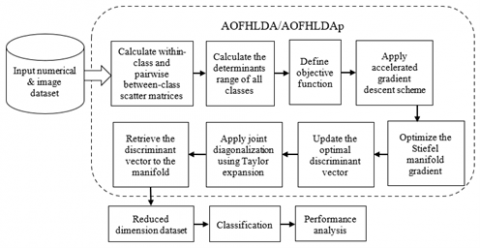
This section provides a brief overview of the AOFHLDA and AOFHLDAp algorithms. It presents a detailed methodology for the AO approach applied to the FHLDA and FHLDAp algorithms. The overall pipeline of these algorithms is illustrated in Figure 1.
3.1 Preliminaries
Let $x \in \mathbb{R}^{p \times n}$ be the given data matrix and $x=$ $\left(x_1, \ldots, x_n\right)$, wherein $p$ is the data dimension and $n$ is the total instances. Additionally, $k$ denotes the class number, $c$ denotes the target subspace dimension, and $K$ denotes the total classes. Let $\mathcal{G} \in \mathbb{R}^{p \times c}$ is a conversion matrix to a $c$ dimensional subspace. The between-class scatter matrix $\left(S_{\ell}\right)$, within-class scatter matrix $\left(S_w\right)$, and the overall scatter matrix $\left(\mathcal{S}_t\right)$ are determined together by the pairwise between-class matrix $\left(\mathcal{B}_{k \ell}\right)$ as in the study by Sreedharan and Nadarajan [13]. In this AOFHLDA algorithm, the discriminant value of all classes is calculated to get the best $\mathcal{G}$. The objective function is given as:
$\min _{\mathcal{G}} \mathcal{J}_1(\mathcal{G})=\sum_{k<l} n_{k} n_{\ell} \frac{\operatorname{Tr}\left(\mathcal{G}^T \mathcal{S}_{w} \mathcal{G}\right)}{\operatorname{Tr}\left(\mathcal{G}^T \mathcal{B}_{k \ell \mathcal{G}}\right),}$ s.t. $\mathcal{G}^T \mathcal{G}=I$ (1)
In Eq. (1), $n_k$ is the total samples in $k$. The gradient of Eq. (1) is given by:
$\begin{gathered}\nabla \mathcal{J}_1 \triangleq \frac{\partial \mathcal{J}_1}{\partial \mathcal{G}}=2 \sum_{k<l} n_k n_{\ell} \frac{\delta_w \mathcal{G}}{\operatorname{Tr}\left(\mathcal{G}^T \mathcal{B}_{k \ell} \mathcal{G}\right)}- \sum_{k<l} n_k n_{\ell} \mathcal{B}_{k \ell} \mathcal{G} \frac{\operatorname{Tr}\left(\mathcal{G}^T \delta_w \mathcal{G}\right)}{\left(\operatorname{Tr}\left(\mathcal{G}^T \mathcal{B}_{k \ell} \mathcal{G}\right)\right)^2}\end{gathered}$ (2)
The constraint $\mathcal{G}^T \mathcal{G}=I$ applies $\mathcal{G}$ on Nesterov’s accelerated gradient descent scheme to get the optimized Stiefel manifold.
3.2 Accelerated gradient descent scheme on the Stiefel manifold for FHLDA
This new accelerated optimization is used to optimize functions on the Stiefel manifold by generalizing the dynamically restart method. But two difficulties must be resolved while applying this scheme to the Stiefel manifold: (i) the non-convexity of the objective function, and (ii) it should obtain an efficient way of generalizing the momentum step to the manifold.
3.2.1 Restart for non-convex functions
While applying an accelerated gradient method on the Stiefel manifold, the problem is occurred that the manifold is compact and thus only the convex functions are constant. So, the functions being optimizing are essentially non-convex. In this scenario, the global convergence is not ensured. Rather, it is observed that in a small neighborhood of a local best $\mathcal{G}^*$, the function can be robustly convex and smooth, given that the Hessian at $\mathcal{G}^*$ is positive definite.
Also, the ratio of the robust convexity and smoothness variables in this neighborhood can be the nearer to the condition number of $\nabla^2 f\left(\mathcal{G}^*\right)$, represented as $\kappa\left(\mathcal{G}^*\right)$.
Therefore, the accelerated gradient scheme recommends that a scheme must be designed that establishes a convergence rate of $O\left(\left(1-\kappa\left(\mathcal{G}^*\right)^{-1 / 2}\right)^t\right)$ after it is nearer to the local minimum $\mathcal{G}^*$. However, because this study copes with functions that are not globally convex, a scheme is designed, which ensures to converge to a local minimum even for non-convex functions, and accomplishes the best convergence rate after it is nearer to the local minimum.
Figure 1. Overall pipeline of the proposed study
The proposed scheme is to alter the function restart method and a below restart criterion is adopted, which forces an adequate reduction in the objective function.
$f\left(g_{t+1}\right)>f\left(g_t\right)-l_R \gamma_t\left\|\nabla f\left(y_t\right)\right\|^2$ (3)
In Eq. (3), $l_R$ denotes a variable, which is small constant, and $\gamma_t$ denotes the step size at step $t$.
This criterion is applied to the optimization issues on the Stiefel manifold, and its convergence for non-convex functions on Euclidean space is analyzed.
Consider $f$ is a differentiable, $L$-smooth function on $\mathbb{R}^n$, i.e., $\nabla f$ is Lipschitz with constant $L$. As well, consider that $f$ is bounded below.
Assume the iteration Eq. (4) with step size $\gamma_t$ selected to satisfy $l /{ }_I \leq \gamma_t \leq \gamma_{t-1}$ for some $l \leq 1$ and $f\left(g_{t+1}\right) \leq$ $f\left(y_t\right)-\left(\gamma_t / 2\right)\left\|\nabla f\left(y_t\right)\right\|_2^2$.
$\begin{gathered}g_0=y_0, g_{t+1}=y_t-\gamma_t \nabla f\left(y_t\right), y_{t+1}=g_{t+1}+ \\ \alpha_t\left(g_{t+1}-g_t\right)\end{gathered}$ (4)
When this iteration is restarted whenever (3) holds, obtain
$\lim _{t \rightarrow \infty}\left\|\nabla f\left(g_t\right)\right\| \rightarrow 0$ (5)
3.2.2 Exploration and interpolation on the Stiefel manifold
Now, it is understood that how to obtain around knowing the robust convexity and smoothness variables and how to cope with non-convex functions in the process. Consider the difficulty of generalizing the momentum step of Eq. (4) to the manifold as:
$\mathcal{Y}_{t+1}=\mathcal{G}_{t+1}+\alpha_t\left(\mathcal{G}_{t+1}-\mathcal{G}_t\right)$ (6)
Consider the difficulty of effectively extrapolating and interpolating on the Stiefel manifold, i.e., given two points $\mathcal{G}, \mathcal{Y} \in S_{p, c}$ and $\alpha \in \mathbb{R}$, it is essential to determine points $(1-\alpha) \mathcal{G}+\alpha \mathcal{Y}$ on a curve via $\mathcal{G}$ and $\mathcal{Y}$. By assigning $\alpha \in$ $(0,1)$, this gives a way of averaging points on the manifold and by assigning $\alpha>1$ or $\alpha<0$, it can extrapolate as in Eq. (6).
A promising method would be to execute the extrapolation or interpolation in Euclidean space and then project back onto the Stiefel manifold. But this estimation process that comprises the orthogonal part from the joint diagonalization-based decomposition of the matrix is highly expensive compared to the proposed algorithm, particularly for large matrices. One could also substitute the estimation by a reorthogonalization process like Gram-Schmidt. But this is fairly improper when k (the number of vectors) is large and is also not as low-cost as this algorithm, which only comprises the matrix products and inversions.
The method for generalizing $(1-\alpha) \mathcal{G}+\alpha \mathcal{Y}$ is to solve for a $V \in\left(T_G S_{p, c}\right)^*$, which satisfies
$\mathcal{Y}=R\left(\mathcal{G}, \phi_q(V)\right), \mathcal{Y}=\mathcal{G}+V$ (7)
In Eq. (7), R is a retraction, which is predetermined. Then, extrapolate or average by assigning
$\begin{gathered}(1-\alpha) \mathcal{G}+\alpha \mathcal{Y}=R\left(\mathcal{G}, \phi_q(\alpha V)\right) \\ (1-\alpha) \mathcal{G}+\alpha \mathcal{Y}=\mathcal{G}+\alpha V\end{gathered}$ (8)
Observe that the utilization of $\phi_q$ enables the algorithm to execute in the dual tangent space. The problem with this solving Eq. (7) for $V$, i.e., finding a $V$ such that $R\left(\mathcal{G}, \phi_q(V)\right)=\mathcal{Y}$ for some given $\mathcal{G}$ and $Y$. But when retraction is considered to be $R_1$, then this solves Eq. (9) for $V$.
$\left(I+\frac{1}{2}\left(V \mathcal{G}^T-\mathcal{G} V^T\right)\right) \mathcal{G}=\left(I-\frac{1}{2}\left(V \mathcal{G}^T-\mathcal{G} V^T\right)\right) \mathcal{Y}$ (9)
Because $\mathcal{G}^T \mathcal{G}=\mathcal{Y}^T \mathcal{Y}=I$, one can simply verify that $V=$ $2 \mathcal{Y}\left(I+\mathcal{G}^T \mathcal{Y}\right)^{-1}$ solves Eq. (8). Here, observing $V \in \mathbb{R}^{p, c}$ as an element of the dual tangent space via the Frobenius inner product. Also, verify that when $V$ is substituted by $V^{\prime}=V+$ $\mathcal{G} S$ for any symmetric $c \times c$ matrix $S$, then $V \mathcal{G}^T-\mathcal{G} V^T=$ $V^{\prime} \mathcal{G}^T-\mathcal{G}\left(\mathcal{G}^{\prime}\right)^T$. This defines that $V^{\prime}$ also satisfies Eq. (9). Particularly, $V$ is substituted by its orthogonal projection onto the dual tangent space $\left(T_G\right)^*$, which then provides the target vector.
One possible problem with this method is the probability that the matrix $\left(I+\mathcal{G}^T \mathcal{Y}\right)$ could be singular or ill-conditioned. To solve this problem, the matrix $\left(I+\mathcal{G}^T \mathcal{Y}\right)$ is wellconditioned providing $\mathcal{G}$ and $\mathcal{Y}$ are not too far apart on $S_{p, c}$. Consider $\mathcal{G}, \mathcal{Y} \in S_{p, c}$. The geodesic distance between $\mathcal{G}$ and $\mathcal{Y}$ w.r.t. the quotient metric as:
$\begin{gathered}d_{S_{p, c}^Q}(\mathcal{G}, \mathcal{Y})^2=\inf _{C(t):[0,1] \rightarrow S_{p, c}} \int_0^1 \operatorname{Tr}\left(C^{\prime}(t)(I-\right. \left.\left.\frac{1}{2} C(t) C(t)^T\right) C^{\prime}(t)^T\right) d t\end{gathered}$ (10)
In Eq. (10), the infimum is taken over each path $C(t)$ that connect $\mathcal{G}$ and $\mathcal{Y}$, i.e., for which $C(0)=\mathcal{G}$ and $C(1)=\mathcal{Y}$. Likewise, the geodesic distance is written w.r.t. the embedding metric as:
$d_{S_{p, c}^E}(\mathcal{G}, \mathcal{Y})^2=\inf _{C(t):[0,1] \rightarrow S_{p, c}} \int_0^1 \operatorname{Tr}\left(C^{\prime}(t) C^{\prime}(t)^T\right) d t$ (11)
In Eq. (11), the infimum is taken over the same set where $C(0)=\mathcal{G}$ and $C(1)=\mathcal{Y}$.
Thus, this method provides computationally efficient algorithm for averaging and extrapolating on the Stiefel manifold.
3.2.3 Gradient restart method
Remember that the gradient restart method reinitiates iteration (4) whenever $\nabla f\left(y_{t-1}\right) \cdot\left(\mathcal{G}_t-\mathcal{G}_{t-1}\right)>0$. Observing that $\mathcal{G}_t=\mathcal{Y}_{t-1}-\gamma_{t-1} \nabla f\left(\mathcal{Y}_{t-1}\right)$ and this criterion is rewritten as:
$-\gamma_{t-1}\left\|\nabla f\left(\mathcal{Y}_{t-1}\right)\right\|_2^2+\nabla f\left(\mathcal{Y}_{t-1}\right) \cdot\left(\mathcal{Y}_{t-1}-\mathcal{G}_{t-1}\right)>0$ (12)
It is observed that on the manifold $\left\|\nabla f\left(\mathcal{Y}_{t-1}\right)\right\|_2^2$ must become $\left\|\nabla f\left(\mathcal{Y}_{t-1}\right)\right\|_{q^*}^2$. Here, seeing $\nabla f\left(\mathcal{Y}_{t-1}\right)$ as an element of the dual tangent space. The difficult part is generalizing $+\nabla f\left(\mathcal{Y}_{t-1}\right) \cdot\left(\mathcal{Y}_{t-1}-\mathcal{G}_{t-1}\right)$. To solve for $V \in\left(S_{y_{t-1}}\right)^*$, the method is presented such that
$\mathcal{G}_{t-1}=R\left(\mathcal{Y}_{t-1}, \phi_q(V)\right)$ (13)
Then, this element $V$ acts as $\mathcal{G}_{t-1}-\mathcal{Y}_{t-1}$ and the correspondent of the gradient restart criterion becomes
$-\gamma_{t-1}\left\|\nabla f\left(\mathcal{Y}_{t-1}\right)\right\|_{q^*}^2-\left\langle\nabla f\left(\mathcal{Y}_{t-1}\right), V\right\rangle_{q^*}>0$ (14)
Eq. (13) can be effectively resolved for V when the retraction is used as $R_1$.
3.2.4 Accelerated gradient descent on the Stiefel manifold
The above-studied concepts are combined to design an accelerated gradient descent scheme with the gradient restart on the Stiefel manifold as in Algorithm 1.
Algorithm 1 Accelerated gradient descent with gradient restart method
Input: Smooth function $f$, tolerance $\epsilon$, initial step size $\gamma_0$, variables needed for line search $\lambda_d, c_L$
Output: A point $\mathcal{G}_t$ such that $\left\|\nabla f\left(\mathcal{G}_t\right)\right\|_{q^*}<\epsilon$
After that, $\mathcal{G}$ is retrieved to the manifold based on the joint diagonalization via Taylor expansion with less computational complexity [13]. Accordingly, the proposed accelerated optimization can achieve faster convergence and reduce the complexity of Stiefel gradient manifolds effectively.
3.3 Accelerated optimization with FHLDAp
For FHLDAp, a pairwise within-class scatter matrix $\left(\mathcal{W}_{k l}\right)$ is also determined along with $\mathcal{B}_{k \ell}$. The objective function for FHLDAp is rewritten as:
$\min _G \mathcal{J}_2(\mathcal{G})=\sum_{k<l} n_k n_{\ell} \frac{\operatorname{Tr}\left(\mathcal{G}^T \mathcal{W}_{k \ell} \mathcal{G}\right)}{\operatorname{Tr}\left(\mathcal{G}^T \mathcal{B}_{k \ell \mathcal{G}}\right)}$, s.t. $\mathcal{G}^T \mathcal{G}=I$ (15)
Similar to the FHLDA, the accelerated gradient descent on the Stiefel manifold is applied to solve (15). Algorithm 2 presents the overall steps in solving Eq. (1) or Eq. (15) iteratively.
Algorithm 2 Accelerated optimization on FHLDA or FHLDAp algorithm
Input: $X \in \mathbb{R}^{p \times n}$, class matrix $\mathcal{Y} \in \mathbb{R}^{n \times K}$ and $c$
putput: Projection matrix $\mathcal{G} \in \mathbb{R}^{p \times c}$
The algorithm initializes the projection matrix $\mathcal{G}$ using standard LDA or trace ratio LDA based on the subspace dimension. It then performs an iterative optimization process using accelerated gradient descent on the Stiefel manifold (Algorithm 1). The optimization is guided by the specified objective function Eq. (1) or Eq. (16), and the resulting $\mathcal{G}$ is retrieved to the manifold using joint diagonalization. The algorithm continues iterating until convergence of the objective function is achieved, aiming to accelerate the optimization process for FHLDA or FHLDAp and potentially enhance convergence speed and overall performance.
Figure 2 illustrates the convergence behavior of various algorithms on the Steifel manifold. It compares the number of iterations to the condition number on a logarithmic scale. The accelerated approach shows superior convergence, with the number of iterations scaling slightly better than the square root of the condition number. Therefore, the accelerated gradient descent with gradient restart method outperforms others, even for small condition numbers.
3.4 Complexity analysis
The proposed algorithm involves joint diagonalization via Taylor expansion for initialization, resulting in a time complexity of $O\left(p^2\right)$. Calculating $\mathcal{S}_w$ takes $O(n p)$ time, while calculating pairwise $\mathcal{B}_{k \ell}$ takes $O(K p)$ time. Each iteration of the while loop, which involves the accelerated gradient descent on the Stiefel manifold based on Algorithm 1 takes $O(\sqrt{p})$ time. Therefore, the total time complexity for Algorithm 2 is $O\left(p^2\right)+O(t \sqrt{p})$, where $t$ is the number of loops until convergence. The proposed AOFHLDA and AOFHLDAp converge quickly, so $t$ is smaller than $p$. In practice, the time complexity for Algorithm 2 is $O\left(p^2\right)$.
3.5 Key improvements and advantages
Key improvements include reducing time complexity, improving convergence rate, and broadening applicability. The accelerated optimization scheme reduces the Stiefel manifold gradient complexity from $O\left(p^2\right)$ to $O(\sqrt{p})$, making it faster and more scalable. The Nesterov accelerated gradient scheme achieves optimal convergence rates for smooth and strongly convex functions on manifolds. The proposed algorithms are applicable to both single-label and multi-label HDDs from diverse domains. These advancements offer faster, more accurate and broadly applicable dimensionality reduction for HDD analysis.
Figure 2. Convergence behavior of different algorithms on Steifel manifold
The subsequent section will focus on the empirical validation of the proposed AOFHLDA and AOFHLDAp algorithms. Extensive experiments are conducted on diverse benchmark datasets including facial images, object images, and video datasets. The performance of AOFHLDA and AOFHLDAp is compared against existing state-of-the-art LDA variants. Evaluation metrics and computational efficiency are reported to fully assess the effectiveness and practical utility of the proposed algorithms. Details including dataset statistics, experimental setup, and parameter tuning, will be provided to ensure transparency and reproducibility of the results.
This section assesses the performance of the proposed AOFHLDA and AOFHLDAp algorithms for dimension reduction in comparison to existing algorithms.
4.1 Experimental setup
Hardware: The experiments were conducted on a Windows 10 64-bit system with 4GB of RAM, a 1TB hard disk, and an Intel® Core™ i5-4210 CPU running at 2.80GHz to ensure consistent and reproducible evaluations.
Software: The proposed AOFHLDA and AOFHLDAp algorithms, along with the existing algorithms (FHLDA [13], FHLDAp [13], ALDA [17], G2DLDA [19], and SMLDA [21]) were implemented in MATLAB 2017b. This ensures a standardized environment for fair comparisons.
Datasets: The evaluation covered both single-label and multi-label classifications using diverse datasets:
The data distribution details for each dataset are provided in [13], ensuring transparency regarding the characteristics of the datasets. In this study, a data split ratio of 80:20 is used to analyze the performance of the proposed and existing algorithms.
Parameter settings: In this experiment, we used the following parameters for the proposed AOFHLDA and AOFHLDAp algorithms: $\epsilon=10^{-10}: \gamma_0=0.1, \lambda_d=1.7$, and $c_L=0.7$. The ALDA and SMLDA algorithms do not require initialization parameters. For G2DLDA, we used regularization $p=0.5$ and nonnegative tuning parameter $\sigma=$0.001.
4.2 Evaluation metrics
The performance of single and multi-label classification using different algorithms is measured regarding the following metrics:
$\begin{gathered}\text { Accuracy }= \frac{\text { True Positive }(T P)+\text { True Negative }(T N)}{T P+T N+\text { False Positive }(F P)+\text { False Negative }(F N)}\end{gathered}$ (16)
In Eq. (16), TP is the total correctly categorized positive labels, FP is the total incorrectly categorized positive labels, FN is the total incorrectly categorized negative labels, and TN is the total correctly categorized negative labels.
Precision $=\frac{T P}{T P+F P}$ (17)
Recall $=\frac{T P}{T P+F N}$ (18)
$F-$ measure $=2 \times \frac{\text { Precision } \text { Recall }}{\text { Precision }+ \text { Recall }}$ (19)
In addition to these metrics, the performance of multi-label classification is measured according to the Hamming Loss (HL), Ranking Loss (RL), 1-Error (1-E), Coverage, and Mean Precision (MP).
The main performance indicators chosen are accuracy, precision, recall, and F-measure. These indicators provide a balanced assessment of different aspects of quality. Accuracy measures overall effectiveness, precision shows the reliability of positive classifications, and recall measures the coverage of actual positives, emphasizing robustness. The F-measure provides a weighted aggregate view of these metrics.
For multi-label settings, additional metrics such as HL, RL, 1-E, coverage, and MP are considered to gain further insight into performance across classes with imbalance. These metrics have been commonly used to evaluate multi-label classifiers in various domains and reveal the model's capabilities in handling label dependencies.
4.3 Statistical analysis
Table 1 shows p-values for single-label classification problems under the null hypothesis, while Table 2 shows p-values for multi-label classification problems under the null hypothesis.
The performance of AOFHLDAp, AOFHLDA, FHLDA, FHLDAp, ALDA, G2DLDA, and SMLDA differs significantly from each other in all cases, except for AOFHLDAp and AOFHLDA, where their performance is statistically similar. Overall, these findings show that AOFHLDAp and AOFHLDA outperform other LDA methods such as FHLDA, ALDA, etc. for both single-label and multi-label classification. The only instance where the differences are not significant is between AOFHLDAp and AOFHLDA, indicating comparable performance.
Table 1. Wilcoxon tests for single-label classification problems
|
Algorithms |
p-value |
Hypothesis |
|
AOFHLDAp vs ALDA |
0.28 |
Rejected |
|
AOFHLDAp vs G2DLDA |
0.31 |
Rejected |
|
AOFHLDAp vs SMLDA |
0.58 |
Rejected |
|
AOFHLDAp vs FHLDA |
0.13 |
Rejected |
|
AOFHLDAp vs FHLDAp |
0.17 |
Rejected |
|
AOFHLDAp vs AOFHLDA |
0.00 |
Not rejected |
|
AOFHLDA vs ALDA |
0.62 |
Rejected |
|
AOFHLDA vs G2DLDA |
0.36 |
Rejected |
|
AOFHLDA vs SMLDA |
0.44 |
Rejected |
|
AOFHLDA vs FHLDA |
0.21 |
Rejected |
|
AOFHLDA vs FHLDAp |
0.15 |
Rejected |
|
FHLDAp vs ALDA |
0.28 |
Rejected |
|
FHLDAp vs G2DLDA |
0.44 |
Rejected |
|
FHLDAp vs SMLDA |
0.19 |
Rejected |
|
FHLDAp vs FHLDA |
0.37 |
Rejected |
|
FHLDA vs ALDA |
0.95 |
Rejected |
|
FHLDA vs G2DLDA |
0.53 |
Rejected |
|
FHLDA vs SMLDA |
0.71 |
Rejected |
|
SMLDA vs ALDA |
0.24 |
Rejected |
|
SMLDA vs G2DLDA |
0.61 |
Rejected |
|
G2DLDA vs ALDA |
0.47 |
Rejected |
Table 2. Wilcoxon tests for multi-label classification problems
|
Algorithms |
p-value |
Hypothesis |
|
AOFHLDAp vs ALDA |
0.71 |
Rejected |
|
AOFHLDAp vs G2DLDA |
0.29 |
Rejected |
|
AOFHLDAp vs SMLDA |
0.43 |
Rejected |
|
AOFHLDAp vs FHLDA |
0.24 |
Rejected |
|
AOFHLDAp vs FHLDAp |
0.19 |
Rejected |
|
AOFHLDAp vs AOFHLDA |
0.00 |
Not rejected |
|
AOFHLDA vs ALDA |
0.35 |
Rejected |
|
AOFHLDA vs G2DLDA |
0.68 |
Rejected |
|
AOFHLDA vs SMLDA |
0.54 |
Rejected |
|
AOFHLDA vs FHLDA |
0.21 |
Rejected |
|
AOFHLDA vs FHLDAp |
0.16 |
Rejected |
|
FHLDAp vs ALDA |
0.39 |
Rejected |
|
FHLDAp vs G2DLDA |
0.52 |
Rejected |
|
FHLDAp vs SMLDA |
0.28 |
Rejected |
|
FHLDAp vs FHLDA |
0.44 |
Rejected |
|
FHLDA vs ALDA |
0.95 |
Rejected |
|
FHLDA vs G2DLDA |
0.61 |
Rejected |
|
FHLDA vs SMLDA |
0.33 |
Rejected |
|
SMLDA vs ALDA |
0.27 |
Rejected |
|
SMLDA vs G2DLDA |
0.66 |
Rejected |
|
G2DLDA vs ALDA |
0.58 |
Rejected |
In conclusion, the Wilcoxon signed-rank test results in Table 1 and Table 2 provide statistical evidence that the proposed AOFHLDAp and AOFHLDA offer significant improvements in accuracy compared to current LDA techniques for single- and multi-label classification tasks, with only minor distinctions between the two proposed algorithms.
4.4 Analysis on single-label classification
Figure 3 depicts the comparison results of various versions of LDA algorithms on the PIE dataset. The proposed AOFHLDA and AOFHLDAp algorithms outperform existing methods in terms of precision, recall, f-measure, and accuracy metrics. The precision of the ALDA, G2DLDA, SMLDA, FHLDA, FHLDAp, AOFHLDA, and AOFHLDAp algorithms is 70.28%, 73.65%, 78.82%, 86.1%, 86.72%, 89.36%, and 90.01%, respectively. The recall of the ALDA, G2DLDA, SMLDA, FHLDA, FHLDAp, AOFHLDA, and AOFHLDAp algorithms is 67.19%, 70.91%, 75.44%, 79.85%, 81.52%, 85.24%, and 86.1%, respectively. The f-measure of the ALDA, G2DLDA, SMLDA, FHLDA, FHLDAp, AOFHLDA, and AOFHLDAp algorithms is 69.28%, 72.25%, 77.09%, 82.57%, 83.75%, 87.25%, and 88.01%, respectively. The accuracy of the ALDA, G2DLDA, SMLDA, FHLDA, FHLDAp, AOFHLDA, and AOFHLDAp algorithms is 65.92%, 70.54%, 76.63%, 83.14%, 86.28%, 90.17%, and 91.28%, respectively.
On average, AOFHLDA achieves absolute improvements of 12.95%, 13.68%, 13.33%, and 17.87% in precision, recall, f-measure, and accuracy respectively. Similarly, AOFHLDAp demonstrates absolute gains of 13.77%, 14.83%, 14.32%, and 19.32% in precision, recall, f-measure, and accuracy respectively. These results highlight the competitive advantage of AOFHLDA and AOFHLDAp in efficiently producing optimal discriminant vectors through accelerated gradient descent on the Stiefel manifold.
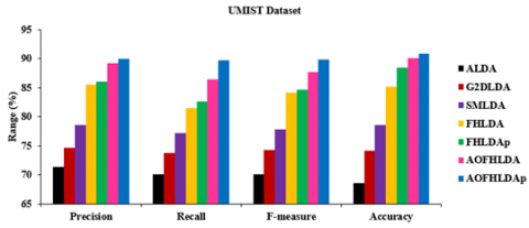
Figure 4 illustrates an assessment of various LDA algorithms on the UMIST dataset, utilizing precision, recall, f-measure, and accuracy metrics. The findings indicate that the proposed AOFHLDA and AOFHLDAp algorithms outperform existing methods. The precision of the ALDA, G2DLDA, SMLDA, FHLDA, FHLDAp, AOFHLDA, and AOFHLDAp algorithms is 71.43%, 74.69%, 78.55%, 85.54%, 86.1%, 89.21%, and 90.04%, respectively. The recall of the ALDA, G2DLDA, SMLDA, FHLDA, FHLDAp, AOFHLDA, and AOFHLDAp algorithms is 70.17%, 73.81%, 77.15%, 81.45%, 82.66%, 86.38%, and 89.74%, respectively. The f-measure of the ALDA, G2DLDA, SMLDA, FHLDA, FHLDAp, AOFHLDA, and AOFHLDAp algorithms is 70.13%, 74.25%, 77.84%, 84.12%, 84.64%, 87.77%, and 89.89%, respectively. The accuracy of the ALDA, G2DLDA, SMLDA, FHLDA, FHLDAp, AOFHLDA, and AOFHLDAp algorithms is 68.56%, 74.13%, 78.57%, 85.23%, 88.42%, 90.15%, and 90.93%, respectively.
On average, AOFHLDA shows absolute improvements of 12.55%, 12.11%, 12.24%, and 14.14% in precision, recall, f-measure, and accuracy, respectively. Similarly, AOFHLDAp achieves absolute gains of 13.65%, 16.47%, 14.95%, and 15.13% on those evaluation metrics. These consistent improvements across multiple metrics demonstrate the ability of AOFHLDA and AOFHLDAp to efficiently reduce dimensionality while preserving discriminative information. By utilizing accelerated optimization on the Stiefel manifold, the algorithms extract higher-quality low-dimensional representations compared to traditional LDA approaches, as indicated by the various evaluation measures.
Figure 3. Comparison of different dimensionality reduction algorithms on PIE dataset
Figure 4. Comparison of different dimensionality reduction algorithms on UMIST dataset
(a)
(b)
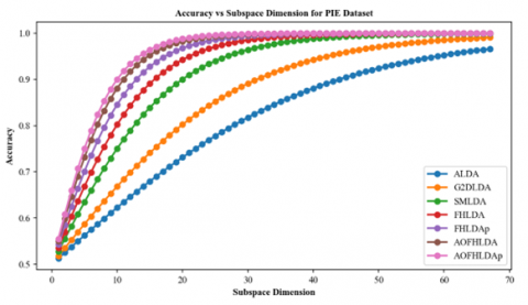
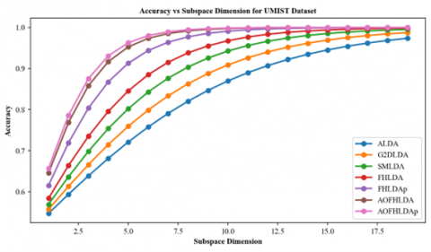
Figure 5. Comparison of accuracy using different subspace dimension $c(c=K-1)$ for single-label classification. (a) PIE dataset and (b) UMIST dataset
Figure 5 displays accuracy results for different subspace dimensions on the PIE and UMIST datasets. The AOFHLDA and AOFHLDAp algorithms consistently achieve higher accuracy compared to other algorithms. Furthermore, the accuracy of AOFHLDA and AOFHLDAp improves as the subspace dimension increases, outperforming other algorithms at higher dimensions. This indicates that AOFHLDA and AOFHLDAp are effective at utilizing larger subspaces to enhance recognition accuracy on the PIE and UMIST datasets.
4.5 Analysis on multi-label classification
Figure 6 illustrates the test results of various LDA algorithms on the Barcelona dataset, indicating that the proposed AOFHLDA and AOFHLDAp outperform existing techniques. The precision of the ALDA, G2DLDA, SMLDA, FHLDA, FHLDAp, AOFHLDA, and AOFHLDAp algorithms is 70.3%, 74.26%, 79.63%, 85.78%, 87.01%, 90.31%, and 91.01%, respectively. The recall of the ALDA, G2DLDA, SMLDA, FHLDA, FHLDAp, AOFHLDA, and AOFHLDAp algorithms is 72.63%, 75.91%, 78.35%, 84.36%, 85.83%, 89.14%, and 91.88%, respectively. The f-measure of the ALDA, G2DLDA, SMLDA, FHLDA, FHLDAp, AOFHLDA, and AOFHLDAp algorithms is 71.61%, 75.08%, 78.98%, 85.64%, 86.42%, 89.72%, and 91.44%, respectively.
The accuracy of the ALDA, G2DLDA, SMLDA, FHLDA, FHLDAp, AOFHLDA, and AOFHLDAp algorithms is 68.63%, 74.95%, 79.47%, 85.41%, 86.01%, 90.45%, and 91.21%, respectively. On average, AOFHLDA achieves absolute improvements of 13.75%, 12.24%, 12.79%, and 14.65% on precision, recall, f-measure, and accuracy metrics, while AOFHLDAp obtains gains of 14.63%, 15.69%, 14.95%, and 15.61% on those metrics. These consistent margins are attributed to the use of accelerated gradient descent on the Stiefel manifold to efficiently reduce data dimensionality while retaining discriminative information.
Figure 7 shows a comparison of different LDA algorithms on the MediaMill dataset. The precision of the ALDA, G2DLDA, SMLDA, FHLDA, FHLDAp, AOFHLDA, and AOFHLDAp algorithms is 72.13%, 75.03%, 79.66%, 85.45%, 86.31%, 90.05%, and 90.84%, respectively. The recall of the ALDA, G2DLDA, SMLDA, FHLDA, FHLDAp, AOFHLDA, and AOFHLDAp algorithms is 68.23%, 72.18%, 77.52%, 83.64%, 84.72%, 88.47%, and 90.6%, respectively. The f-measure of the ALDA, G2DLDA, SMLDA, FHLDA, FHLDAp, AOFHLDA, and AOFHLDAp algorithms is 70.41%, 73.58%, 78.58%, 84.67%, 85.51%, 89.25%, and 90.72%, respectively. The accuracy of the ALDA, G2DLDA, SMLDA, FHLDA, FHLDAp, AOFHLDA, and AOFHLDAp algorithms is 68.17%, 74.94%, 78.81%, 83.45%, 85%, 90%, and 90.91%, respectively.
On average, the precision of AOFHLDA and AOFHLDAp is 12.96% and 13.95% higher, respectively, than the other LDA algorithms. The recall of AOFHLDA and AOFHLDAp is 14.51% and 17.27% greater, respectively, than the other LDA algorithms. The f-measure of AOFHLDA and AOFHLDAp is 13.62% and 15.49% higher, respectively, than the other LDA algorithms. The accuracy of AOFHLDA and AOFHLDAp is 15.28% and 16.44% higher, respectively, than the other LDA algorithms. Therefore, it is evident that the AOFHLDA and AOFHLDAp algorithms achieve better efficiency on the MediaMill dataset by reducing data dimensionality for classification.
Figure 8 illustrates the comparison of the complexity of different LDA algorithms on various datasets in terms of runtime. AOFHLDAp demonstrates lower runtimes compared to ALDA, G2DLDA, SMLDA, FHLDA, FHLDAp, and AOFHLDA by 32.12%, 27.7%, 15.68%, 9.9%, 6.3%, and 3.27% on the PIE dataset, 29.81%, 26.26%, 20.07%, 14.79%, 7.98%, and 0.9% on the UMIST dataset, 45.09%, 37.7%, 34.83%, 23.23%, 22.17%, and 2.68% on the MediaMill dataset, and 34.07%, 26.45%, 21.93%, 16.82%, 9.18%, and 4.3% on the Barcelona dataset. This consistent improvement in runtime across all datasets demonstrates the effectiveness of the proposed AO approach in optimizing the computational efficiency of the FHLDA and FHLDAp algorithms, which can have significant implications for real-world applications where processing time is critical.
Figure 6. Comparison of different dimensionality reduction algorithms on Barcelona dataset
Figure 7. Comparison of different dimensionality reduction algorithms on MediaMill dataset
Figure 8. Comparison of runtime for different dimensionality reduction algorithms on various datasets
(a)
(b)
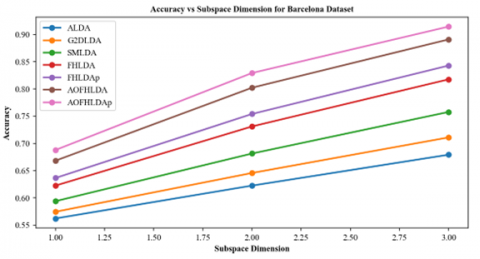
Figure 9. Comparison of accuracy using different subspace dimension $c(c=K-1)$ for multi-label classification. (a) Barcelona dataset and (b) MediaMill dataset
Table 3. Comparison of different LDA algorithms for multi-label classification
|
Dataset |
Metrics |
ALDA |
G2DLDA |
SMLDA |
FHLDA |
FHLDAp |
AOFHLDA |
AOFHLDAp |
|
Barcelona |
HL |
0.349 |
0.333 |
0.305 |
0.268 |
0.253 |
0.231 |
0.227 |
|
RL |
0.267 |
0.249 |
0.227 |
0.194 |
0.181 |
0.169 |
0.160 |
|
|
1-E |
0.105 |
0.082 |
0.070 |
0.052 |
0.046 |
0.035 |
0.029 |
|
|
Coverage |
2.215 |
2.194 |
2.151 |
2.019 |
2.005 |
1.988 |
1.925 |
|
|
MP |
0.792 |
0.811 |
0.855 |
0.916 |
0.928 |
0.936 |
0.944 |
|
|
MediaMill |
HL |
0.085 |
0.067 |
0.054 |
0.041 |
0.036 |
0.028 |
0.020 |
|
RL |
0.114 |
0.099 |
0.086 |
0.078 |
0.069 |
0.047 |
0.040 |
|
|
1-E |
0.142 |
0.130 |
0.122 |
0.114 |
0.105 |
0.092 |
0.085 |
|
|
Coverage |
25.50 |
25.29 |
25.17 |
25.06 |
24.97 |
24.11 |
23.96 |
|
|
MP |
0.655 |
0.683 |
0.696 |
0.712 |
0.724 |
0.741 |
0.753 |
Figure 9 displays accuracy results for different subspace dimensions on the Barcelona and MediaMill datasets. The AOFHLDA and AOFHLDAp algorithms consistently achieve higher accuracy compared to other algorithms. Furthermore, the accuracy of AOFHLDA and AOFHLDAp improves as the subspace dimension increases, outperforming other algorithms at higher dimensions. This indicates that AOFHLDA and AOFHLDAp are effective at utilizing larger subspaces to enhance recognition accuracy on the Barcelona and MediaMill datasets.
Table 3 presents the results of HL, RL, 1-E, coverage, and MP for different LDA algorithms on the Barcelona and MediaMill datasets. From these analyses, it is concluded that the proposed AOFHLDA and AOFHLDAp algorithms attain a minimum HL, RL, 1-E, coverage, and a maximum MP than the other LDA algorithms with the help of AO on the Stiefel manifold during data dimensionality reduction.
4.5.1 Discussion
The study could benefit from further analysis of how the proposed AOFHLDA and AOFHLDAp algorithms handle label dependencies in multi-label classification. This could involve updating the discrimination objective function and gradient descent optimization to minimize the correlation between uncorrelated labels and maximize the correlation between correlated labels. Additionally, label dependency graphs or association rules could be used to directly model label relationships and inform specialized regularizers or constraints during the optimization process. The algorithms could also be coupled with multi-task learning frameworks to learn multiple models with shared and distinct parameters, accounting for inter-label dependencies. Finally, performance could be evaluated on real-world multi-label datasets with known label correlations to quantify accuracy gains over traditional LDA algorithms.
This study introduces a Nesterov accelerated gradient descent scheme on the Stiefel manifold for optimizing functions with orthogonality constraints. The approach achieves faster convergence rates compared to traditional gradient descent methods by using momentum and an optimized step size sequence. By leveraging the geometry of the Stiefel manifold, it can elegantly handle the enforcement of orthogonality constraints during optimization. The proposed AOFHLDA and AOFHLDAp algorithms apply this scheme to efficiently search for the most discriminative vectors for dimensionality reduction. The accuracy results on multiple benchmark datasets show that this methodology enables superior dimensionality reduction performance compared to other methods. The proposed algorithms achieved over 90% accuracy on all test datasets, compared to ALDA, G2DLDA, SMLDA, FHLDA, and FHLDAp. These algorithms can extract low-dimensional representations for diverse conditions, enabling accurate applications such as automated video tagging, face recognition, etc. The optimization approach produces discriminant projections for complex dimensionality reduction tasks, with the potential to enhance automated analysis in various fields.
The proposed algorithms extract features that are used in a separate classifier. However, this two-step process may hinder classification performance. Future work could explore an end-to-end model that optimizes feature extraction and prediction together, integrating the proposed algorithms into deep learning methods to improve HDD classification.
[1] Georgiou, T., Liu, Y., Chen, W., Lew, M. (2020). A survey of traditional and deep learning-based feature descriptors for high dimensional data in computer vision. International Journal of Multimedia Information Retrieval, 9(3): 135-170. https://doi.org/10.1007/s13735-019-00183-w
[2] Samadi, M., Kiefer, S., Fritsch, S.J., Bickenbach, J., Schuppert, A. (2022). A training strategy for hybrid models to break the curse of dimensionality. Plos One, 17(9): 1-22. https://doi.org/10.1371/journal.pone.0274569
[3] Van Engelen, J.E., Hoos, H.H. (2020). A survey on semi-supervised learning. Machine Learning, 109(2): 373-440. https://doi.org/10.1007/s10994-019-05855-6
[4] Pes, B. (2020). Ensemble feature selection for high-dimensional data: A stability analysis across multiple domains. Neural Computing and Applications, 32(10): 5951-5973. https://doi.org/10.1007/s00521-019-04082-3
[5] Chung, S., Abbott, L.F. (2021). Neural population geometry: An approach for understanding biological and artificial neural networks. Current Opinion in Neurobiology, 70: 137-144. https://doi.org/10.1016/j.conb.2021.10.010
[6] Piironen, J., Paasiniemi, M., Vehtari, A. (2020). Projective inference in high-dimensional problems: prediction and feature selection. Electronic Journal of Statistics, 14: 2155-2197. https://doi.org/10.1214/20-EJS1711
[7] Mosavi, A., Sajedi Hosseini, F., Choubin, B., Goodarzi, M., Dineva, A.A., Rafiei Sardooi, E. (2021). Ensemble boosting and bagging based machine learning models for groundwater potential prediction. Water Resources Management, 35: 23-37. https://doi.org/10.1007/s11269-020-02704-3
[8] Bhattacharjee, P., Mitra, P. (2021). A survey of density based clustering algorithms. Frontiers of Computer Science, 15: 1-27. https://doi.org/10.1007/s11704-019-9059-3
[9] Nanga, S., Bawah, A.T., Acquaye, B.A., Billa, M.I., Baeta, F.D., Odai, N.A., Nsiah, A.D. (2021). Review of dimension reduction methods. Journal of Data Analysis and Information Processing, 9(3): 189-231. https://doi.org/10.4236/jdaip.2021.93013
[10] Vachharajani, B., Pandya, D. (2022). Dimension reduction techniques: Current status and perspectives. Materials Today: Proceedings, 62: 7024-7027. https://doi.org/10.1016/j.matpr.2021.12.549
[11] Ayesha, S., Hanif, M.K., Talib, R. (2020). Overview and comparative study of dimensionality reduction techniques for high dimensional data. Information Fusion, 59: 44-58. https://doi.org/10.1016/j.inffus.2020.01.005
[12] Zheng, S., Ding, C., Nie, F., Huang, H. (2018). Harmonic mean linear discriminant analysis. IEEE Transactions on Knowledge and Data Engineering, 31(8): 1520-1531. https://doi.org/10.1109/TKDE.2018.2861858
[13] Sreedharan, S., Nadarajan, R. (2022). A fast harmonic mean linear discriminant analysis for dimensionality reduction. International Journal of Intelligent Engineering & Systems, 15(4): 216-226. https://doi.org/10.22266/ijies2022.0831.20
[14] Li, Y., Chai, Y., Zhou, H., Yin, H. (2021). A novel dimension reduction and dictionary learning framework for high-dimensional data classification. Pattern Recognition, 112: 1-39. https://doi.org/10.1016/j.patcog.2020.107793
[15] Zhao, G., Zhou, Z., Zhang, J. (2021). Theoretical framework in graph embedding-based discriminant dimensionality reduction. Signal Processing, 189: 1-12. https://doi.org/10.1016/j.sigpro.2021.108289
[16] Qu, H., Li, L., Li, Z., Zheng, J. (2021). Supervised discriminant Isomap with maximum margin graph regularization for dimensionality reduction. Expert Systems with Applications, 180: 1-14. https://doi.org/10.1016/j.eswa.2021.115055
[17] Lu, R., Cai, Y., Zhu, J., Nie, F., Yang, H. (2021). Dimension reduction of multimodal data by auto-weighted local discriminant analysis. Neurocomputing, 461: 27-40. https://doi.org/10.1016/j.neucom.2021.06.035
[18] Su, B., Zhou, J., Wen, J.R., Wu, Y. (2021). Linear and deep order-preserving Wasserstein discriminant analysis. IEEE Transactions on Pattern Analysis and Machine Intelligence, 44(6): 3123-3138. https://doi.org/10.1109/TPAMI.2021.3050750
[19] Li, C.N., Shao, Y.H., Chen, W.J., Wang, Z., Deng, N.Y. (2021). Generalized two-dimensional linear discriminant analysis with regularization. Neural Networks, 142: 73-91. https://doi.org/10.1016/j.neunet.2021.04.030
[20] Zhou, R., Gao, W., Ding, D., Liu, W. (2022). Supervised dimensionality reduction technology of generalized discriminant component analysis and its kernelization forms. Pattern Recognition, 124: 1-35. https://doi.org/10.1016/j.patcog.2021.108450
[21] Xu, L., Raitoharju, J., Iosifidis, A., Gabbouj, M. (2022). Saliency-based multilabel linear discriminant analysis. IEEE Transactions on Cybernetics, 52(10): 10200-10213. https://doi.org/10.1109/TCYB.2021.3069338
[22] Sim, T., Baker, S., Bsat, M. (2002). The CMU pose, illumination, and expression (PIE) database. In: Proceedings of Fifth IEEE International Conference on Automatic Face Gesture Recognition, Washington, DC, USA, pp. 53-58. https://doi.org/10.1109/AFGR.2002.1004130
[23] Lu, J., Plataniotis, K.N., Venetsanopoulos, A.N. (2003). Face recognition using LDA-based algorithms. IEEE Transactions on Neural Networks, 14(1): 195-200. https://doi.org/10.1109/TNN.2002.806647
[24] Snoek, C.G., Worring, M., Van Gemert, J.C., Geusebroek, J.M., Smeulders, A.W. (2006). The challenge problem for automated detection of 101 semantic concepts in multimedia. In Proceedings of the 14th ACM International Conference on Multimedia, pp. 421-430. https://doi.org/10.1145/1180639.1180727
[25] Zheng, S., Ding, C. (2014). Kernel alignment inspired linear discriminant analysis. In: Machine Learning and Knowledge Discovery in Databases: European Conference, Springer Berlin Heidelberg, Springer, Berlin, Heidelberg, pp. 401-416. https://doi.org/10.1007/978-3-662-44845-8_26