Besma Senaï*![]() | Sidi Ahmed Hebri Rahal
| Sidi Ahmed Hebri Rahal![]() | Salim Khiat
| Salim Khiat![]()
© 2023 IIETA. This article is published by IIETA and is licensed under the CC BY 4.0 license (http://creativecommons.org/licenses/by/4.0/).
OPEN ACCESS
The classification of mammographic tumors from medical imagery, a critical step in pathology detection and diagnosis, is addressed in this study. A novel supervised hybrid model that integrates deep learning and machine learning techniques is proposed for the classification of semantically relevant tissue areas. This new approach seeks to overcome the prevalent issue of suboptimal accuracy in conventional mammography tumor prediction methods. In the initial stage, an architecture akin to VGGNet19, EfficientNetB7, InceptionV3, ResNet152, DenseNet201, and MobileNetV2 Convolutional Neural Networks (CNNs) is employed, serving as an automatic feature extractor from medical images. These extracted features are then learned by various classifiers, including K-Nearest Neighbor (KNN), Random Forest (RF), AdaBoost, Support Vector Machine (SVM), and Xgboost, for mammographic tumor classification. This study identifies the most effective CNN model for the intended task. Statistical results demonstrate that the combination of pre-trained CNN models and supervised classification algorithms can significantly enhance efficiency in medical image analysis, particularly in mammographic tumor detection. The proposed model, dubbed EfficientNetB7-Xgboost, utilizes the EfficientNetB7 CNN model for feature extraction and the Xgboost algorithm for classification. However, hyperparameters settings can impact the performance of the EfficientNetB7-Xgboost model. To address this, the Cuckoo Search (CS) algorithm is employed in the subsequent stage to optimize Xgboost hyperparameters. This method is chosen for its known proficiency in eschewing local minimum values, a common issue with conventional parameter optimization approaches. The proposed EfficientNetB7-CS-Xgboost model's performance is validated using mammography data from the DDSM and MIAS datasets. Evaluation metrics include precision, recall, accuracy, and the f1-score. The results are compared against those obtained using EfficientNetB7-Xgboost in conjunction with the particle swarm optimization approach. Experimental findings indicate that coupling EfficientNetB7-Xgboost with the CS algorithm yields superior mammographic tumor prediction results compared to previous models.
image mining, medical image classification, machine learning, Xgboost, Convolutional Neural Networks, Softmax, mammographic
Breast cancer, recognized as the most prevalent cancer in women and the second leading cause of cancer-related deaths, necessitates an urgent need for robust and efficient diagnostic methods. Mammography, a widely utilized medical imaging technique, has proven instrumental in early diagnosis, thereby improving treatment outcomes. However, the escalating volume of mammography images demands swift and precise classification methods for effective large-scale population screening. This paper seeks to address this pressing need by proposing an advanced image classification model leveraging both deep learning and machine learning algorithms [1, 2].
Contemporary classifiers such as Support Vector Machine (SVM) [3], K-nearest neighbor (KNN) [4, 5], Random Forest (RF) [6], AdaBoost [7], Xgboost [8], and Convolutional Neural Network (CNN) [9] have demonstrated significant efficacy in medical image classification. Nevertheless, the complexity and diversity of medical image data perpetually challenge these methods, underscoring the need for refinement.
Deep Neural Networks (DNNs), capable of intricate function approximation, have shown promise in various domains including facial recognition, object detection, and image classification. Their ability to efficiently extract features and perform classification elucidates their potential applicability in mammographic image classification. However, their complex structure, training difficulty, and high processing costs often impede their efficient implementation.
In conventional medical image classification tasks, feature extraction is a crucial yet time-consuming process, with the quality of extracted features dramatically impacting classification performance. CNN, a type of DNN, has excelled in feature extraction for various applications such as sentiment classification [10], demonstrating its potential for mammographic image classification. However, traditional classifiers linked to CNN often fail to comprehend the extracted features fully, thus limiting classification accuracy.
Addressing these challenges, our study's first contribution is the integration of a CNN model and a machine learning algorithm, both exhibiting exceptional performance in medical image classification. We evaluate several pre-trained CNN models, including VGGNet19 [11], EfficientNetB7 [12], InceptionV3 [13], ResNet152 [14], DenseNet201 [15], and MobileNetV2 [16], in tandem with various classifiers such as KNN, SVM, AdaBoost, Xgboost, and RF for tumor classification in mammography images.
The experimental results, in the validation process of the optimal CNN model, show that the EfficientNetB7 model obtains the highest scores among all the pre-trained models used in combination with the Xgboost algorithm in the automatic medical image classification process. The results of this first study involve a novel image classification model called EfficientNetB7-Xgboost to increase the performance of medical image classification. The proposed model achieves improved results by incorporating EfficientNetB7 as a trainable feature extractor to automatically get features from the input and using Xgboost as a high-level recognition network to generate results. This two-step model ensures efficient feature extraction and classification.
However, in a machine learning model, their parameters affect their effectiveness to a large extent. Indeed, the Xgboost model has many hyperparameters and human experience is required to determine the optimal parameters, which increases the difficulty of the model. Nevertheless, the learning efficiency and generalization ability of Xgboost is related to the selection of appropriate parameters. The parameters have a direct impact on the efficiently of the model predictions. Therefore, evolutionary algorithms may be the solution to this challenge. In fact, particle swarm optimization [17], genetic algorithm [18], and ant colony algorithm [19] have been approved to improve the parameters of Xgboost model. However, the particle swarm optimization model and the genetic algorithm fall quickly into local extremes. The three principal limitations of the algorithm are the exploration ratio, the stagnation stage and the convergence speed of the algorithm. On the other hand, recently, the cuckoo search algorithm (CS cuckoo search) is an evolutionary algorithm proposed [20]; it has the advantage of strong global search capability, few parameters and a nice search path and it is efficient to solve multi-objective problems. Motivated by the above facts, the second contribution of this article is the combination of the CS algorithm and the Xgboost algorithm to optimize the hyperparameters of Xgboost.
In this paper, a tumor mammography prediction model based on EfficientNetB7-CS-Xgboost is proposed. The principal contributions of this paper are as follows:
Section 2 of this paper discusses related work, while Section 3 provides a detailed description of the proposed algorithm. Section 4 details the mammography image datasets used, presents the analysis results, and highlights some limitations of our approach. Section 5 concludes the paper and suggests potential future directions.
The current landscape of medical image analysis has been significantly transformed by the advent and growth of machine learning methodologies, particularly Convolutional Neural Networks (CNNs). Ker et al. [21] underscored the potential of CNNs in automatically discovering meaningful hierarchical relationships within data, thereby eliminating the need for manual feature extraction. They comprehensively explored the primary research areas and applications of medical image analysis, including classification, detection, segmentation, registration, and localization.
A trend observed in this field is the utilization of pre-trained CNNs in conjunction with supervised classification algorithms for medical image analysis. Varshni et al. [22] proposed a two-step approach in which pre-trained CNN models were initially employed for feature extraction, followed by the application of various classifiers for distinguishing between normal and abnormal chest radiographs. Their investigation showed that the combination of DenseNet-169 and the Support Vector Machine (SVM) algorithm was optimal, especially for pneumonia detection in chest X-ray images.
Building on the idea of feature extraction through CNNs, Dubrovina et al. [23] suggested using convolutional layers instead of conventional fully connected layers to expedite the class prediction process at the pixel level. Their method, validated on annotated mammography images, demonstrated promising results in tissue classification and image segmentation.
An essential aspect of the feature extraction process is the validation of extracted characteristics before their submission to classification. Arevalo et al. [24] emphasized this factor in their study, demonstrating that their model outperformed previous models by achieving an area under the Receiver Operating Characteristic (ROC) curve between 79.9% and 86%.
To enhance the accuracy of trained CNN models and reduce the re-training time, Lee et al. [25] proposed a model comprising two phases: feature generation via a CNN model and subsequent application of the AdaBoost algorithm to combine Softmax classifiers into recognizable images. This work underscored the potential of combining CNNs with the AdaBoost algorithm to improve image analysis performance.
Following these works, it is noticeable that several studies combined CNN models with machine learning approaches for improved results. For example, Varshni et al. [22] employed the SVM algorithm for classification, while Lee et al. [25] utilized the AdaBoost algorithm. The present study adopts the enhanced AdaBoost algorithm, known as XGBoost, for the classification stage, evaluated through a series of experiments.
Nevertheless, the efficacy of the XGBoost algorithm is largely dependent on its parameters. Efforts have been made to optimize these parameters, as in the study by Zhang et al. [26], where a Particle Swarm Optimization (PSO) was performed to improve the XGBoost hyperparameters. The proposed PSO-XGBoost model outperformed other models in predicting explosion-induced peak particle velocity (PPV).
Other approaches [27], have used the genetic algorithm in tandem with XGBoost to improve model parameters. The authors of this study proposed a novel algorithm for pedestrian detection in images, involving the description of pedestrians by tandem fusion by Histogram of Oriented Gradients (HOG) and Local Binary Patterns (LBP) features, followed by the application of the Genetic Algorithm-XGBoost (GA-XGBoost) algorithm.
Motivated by the efficiency of the Cuckoo Search algorithm in optimization problems, this study proposes its combination with the XGBoost algorithm, detailed in the following section. The hybridization of the Cuckoo Search algorithm and XGBoost aims to enhance classification efficiency.
The objective of this section is to present the novel approach and evaluate the results. This study consists of classification of mammography images that detects abnormalities at an early stage. This section experiments with transfer learning using pre-trained convolutional neural network models and some classifiers to enhance the accuracy of results.
(a) 1st Contribution: A comprative study
(b) 2nd Contribution: Optimized cuckoo search
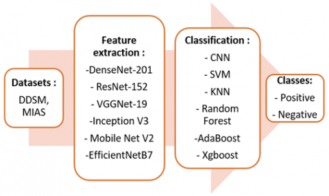
Figure 1. The proposed approach framework
The image dataset and the process used to classify mammograms into two classes (positive and negative) are shown in Figure 1 and are presented in detail in the next sub-sections. In the first sub-section, a description of the images acquired from the Mammographic Institute Society Analysis (MIAS) and Breast Cancer Image (CBIS-DDSM) datasets is provided and the preprocessing applied to these images is described. The objective of the second sub-section is to test some methods and approaches in order to establish a comparative table showing the accuracy rates of each method, which is the first contribution of this paper (see Figure 1 (a)). Finally, the third sub-section presents the Xgboost classifier optimized with the Cuckoo search algorithm which is the second contribution of this study (see Figure 1 (b)).
3.1 Datasets preprocessing
3.1.1 DDSM mammography dataset
The dataset is composed of images from the DDSM [28] and CBIS-DDSM: Breast Cancer Image Dataset [29] databases. The images were preprocessed and transformed to 299×299 images by extracting the ROIs. The data are saved in tfrecords files for TensorFlow. The data set which includes 55,890 training examples (14% positive, 86% negative) are saved in 5 tfrecords files.
The data was split into training and test data. However, this split was done improperly, since the test nimpy files include only masses and the validation files include only calcifications. Therefore, these files must be used together to obtain complete and balanced test data.
- Preprocessing
The dataset is the combination of positive images from the CBIS-DDSM data and negative images from the DDSM data. These data were pre-processed to be converted to 299×299 images. The negative images (DDSM) were divided into 598×598 tiles and resized to 299×299.
The ROIs from the positive images (CBIS-DDSM) were selected using the masks with a small amount of fill to obtain context. Each one of the ROIs was then randomly cropped thrice into 598×598 images with random flipping and rotation, and resized to 299×299 to pass them into the CNN models.
The images are annotated with two stickers:
- Stickers normal 0 for negative and 1 for positive.
- Stickers complete multiclass labels, 0 for negative, 1 for benign calcification, 2 for benign mass, 3 for malignant calcification, 4 for malignant mass.
3.1.2 MIAS
The Mammographic Institute Society Analysis (MIAS) database [30] has mammogram images with a size of 1024×1024 pixels and a resolution of 200 microns. It included 322 mammograms of the right and left breasts of 161 patients, of which 54 were diagnosed as malignant, 69 as benign, and 207 as normal. It included also a file that lists the mammograms in the MIAS database and achieves appropriate details, such as the class of abnormality, the xy coordinates of the image of the center of the abnormality, the approximate radius (in microns) of the abnormality, and the approximate radius (in pixels) of a circle surrounding the abnormality. Site anomalies are classified according to the type of anomaly found (circumscribed masses, calcification, distortions of circumscribed masses, asymmetries, architectural distortions and other well-defined masses). Table 1 shows the column details.
Table 1. MIAS database description
|
Column |
Detail |
|
1st |
MIAS Database reference number |
|
2nd |
Character of background tissue: F-Fatty G-Fatty-glandular D-Dense-glandular |
|
3rd |
Class of abnormality present: 1 CALC-Calcification 2 CIRC-Well-defined/circumscribed masses 3 SPIC-Spiculated masses 4 MIS-Other, ill-defined masses 5 ARCH-Architectural distortion 6 ASYM-Asymmetry 7 NORM-Normal |
|
4th |
Severity of abnormality; B- Benign M-Malignant |
|
5th, 6th |
X y image-coordinates of center of abnormality |
|
7th |
Approximate radius (in pixels) of a circle enclosing the abnormality |
- Preprocessing
Data augmentation: Rotating the images 8 degrees 45 times. These transformations are one of the general principles of training scalable networks with small data sets. Finally, all images were resized to 224×224 to run in the CNN models.
3.2 Comparative study between CNN architectures and classification algorithms
This study consists of two essential parts, starting with feature extraction from mammography images by applying different CNN architectures. Then, the classification of the feature vector obtained in the previous step using different machine learning algorithms to obtain the corresponding class (Figure 2).
Figure 2. Comparative study of classification algorithms
3.2.1 Feature extraction
This step consists in extracting from the mammography images the features that will be used in the classification step. Indeed, this operation is a difficult task that needs a high expertise level and requires a lot of work and time. In addition, the solutions may not be representative because the characteristics obtained are problem specific. In deep neural network models, feature extraction is done automatically by the layers of the CNN. Indeed, the basic features (such as: edges and contours) are generated by the lower layers, while information about the color and shape of the image are obtained by the intermediate layers. In addition, these networks include a fully connected layer for classification. In this work, this fully connected layer is removed in order to obtain a feature vector as output of the network. Hence, the role of the CNN is limited to extracting features automatically only (see Figure 2). The selected architectures to perform the experiment are EfficientNetB7, vgg19, InceptionV3, ResNet152, DenseNet201 and MobileNetV2. The pre-trained weights that were performed to the networks were trained on the ImageNet database.
3.2.2 Features classification
This experiment consists of six cases.
The first case implements the Xgboost classifier on the mammogram features extracted from the CNN model. The parameters applied in this case are the default parameters.
The second case implements the SVM classifier on the CNN features of the mammograms. The SVM maps the input vector of data to a higher dimensional feature space where a maximum margin hyperplane is built. This case uses the default parameters of SVM.
The third case utilizes the fully connected (dense) layer with the Softmax activation function on the CNN in order to distinguish between positive and negative mammograms.
The fourth case applies the Random Forest (RF) classifier on the mammogram features extracted from the CNN. RF is a learning method that applies the average prediction score of a single tree in a combination of multiple decision trees. The settings applied in RF are the default settings. The fifth case applies the AdaBoost classifier in addition to the CNN features. The AdaBoost algorithm is a sequential boosting ensemble learning method in which each weak classifier is modified based on the instances misclassified by all previous classifiers. Its final Decision is the weighted sum of the scores of the results of a combination of the final classifiers. In AdaBoost algorithm the decision tree is applied as the base classifier and the parameters applied are the default parameters. The sixth case applies the K nearest neighbors (KNN) to classify the target points (unknown class) based on their distance from the points making up a training sample.
3.3 Optimization Xgboost
3.3.1 Training process of Xgboost
After the feature extraction step, several classifiers such as Random Forest, Support Vector Machine, etc. were performed for the classification task. But in this paper, the best results were found with Xgboost model as the classifier for the problem. The description of the XGBoost [31] core is as follows:
Let $\mathrm{D}=\left\{\left(\mathrm{x}_{\mathrm{i}}, \mathrm{y}_{\mathrm{i}}\right)\right\}\left(|\mathrm{D}|=\mathrm{n}, \mathrm{x}_{\mathrm{i}} \in \mathbb{R}^{\mathrm{m}}, \mathrm{y}_{\mathrm{i}} \in \mathbb{R}^{\mathrm{n}}\right)$ describes a dataset with $\mathrm{n}$ examples and $\mathrm{m}$ features.
Eq. (1) consists of a tree boosting model output $\hat{\mathrm{y}}_{\mathrm{i}}$ with K trees [32].
$\hat{\mathrm{y}}_{\mathrm{i}}=\sum_{\mathrm{k}=1}^{\mathrm{K}} \mathrm{f}_{\mathrm{k}}\left(\mathrm{x}_{\mathrm{i}}\right), \mathrm{f}_{\mathrm{k}} \in \mathrm{F}$ (1)
where, $\left.\mathrm{F}=\{\mathrm{f}(\mathrm{x})) \omega_{\mathrm{q}}(\mathrm{x})\right\}\left(\mathrm{q}: \mathbb{R}^{\mathrm{m}} \rightarrow \mathrm{T}, \omega \in \mathbb{R}^{\mathrm{T}}\right)$ is the spatial regression or classification trees. Each fk splits a tree into structure part q and leaf weights part ω. T is the number leaves in the tree.
To minimize the following objective function [32], the tree model functions fk can be learned:
$\mathfrak{L}^{(\mathrm{t})}=\sum_{\mathrm{i}=1}^{\mathrm{n}} \mathrm{l}\left(\mathrm{y}_{\mathrm{i}}, \hat{\mathrm{y}}_{\mathrm{i}}^{(\mathrm{t}-1)}+\mathrm{f}_{\mathrm{t}}\left(\mathrm{X}_{\mathrm{i}}\right)\right)+\Omega\left(\mathrm{f}_{\mathrm{t}}\right)$ (2)
where, the term l in Eq. (2) is a training loss function which measures the distance between the prediction $\hat{y}_i$ and the object yi. And Ω represents the penalty term of the tree model complexity [32].
$\Omega\left(f_t\right)=\gamma \mathrm{T}+\frac{1}{2} \lambda \sum_{j=1}^{\mathrm{T}} \omega_{\mathrm{j}}^2$ (3)
Xgboost approximates Eq. (2) using the second order Taylor expansion and the final objective function at step t can be simplified as [32]:
$\mathfrak{L}^{(\mathrm{t})} \simeq \sum_{\mathrm{i}=1}^{\mathrm{n}} \mathrm{l}\left(\mathrm{y}_{\mathrm{i}}, \hat{\mathrm{y}}_{\mathrm{i}}^{(\mathrm{t}-1)}+\mathrm{g}_{\mathrm{i}} \mathrm{f}_{\mathrm{t}}\left(\mathrm{X}_{\mathrm{i}}\right)+\frac{1}{2} \mathrm{~h}_{\mathrm{i}} \mathrm{f}_{\mathrm{t}}^2\left(\mathrm{X}_{\mathrm{i}}\right)\right)+\Omega\left(\mathrm{f}_{\mathrm{t}}\right)$ (4)
where, gi and hi are the first and the second order gradient statistics on the loss function [32].
$\mathrm{g}_{\mathrm{i}}=\partial_{\hat{y}_{\mathrm{i}}^{(\mathrm{t}-1)}} \quad\mathrm{l}\left(\mathrm{y}_{\mathrm{i}}, \hat{\mathrm{y}}_{\mathrm{i}}^{(\mathrm{t}-1)}\right), \mathrm{h}_{\mathrm{i}}=\partial_{\hat{y}_{\mathrm{i}}^{(\mathrm{t}-1)}} \quad\mathrm{l}\left(\mathrm{y}_{\mathrm{i}}, \hat{\mathrm{y}}_{\mathrm{i}}^{(\mathrm{t}-1)}\right)$ (5)
After removing the constant term and expanding Ω, Eq. (4) can be rewritted as [32]:
$\widetilde{\mathfrak{L}^{(t)}}=\sum_{\mathrm{i}=1}^{\mathrm{n}}\left[\mathrm{g}_{\mathrm{i}} \mathrm{f}_{\mathrm{t}}\left(\mathrm{X}_{\mathrm{i}}\right)+\frac{1}{2} \mathrm{~h}_{\mathrm{i}} \mathrm{f}_{\mathrm{t}}^2\left(X_{\mathrm{i}}\right)\right]+\gamma \mathrm{T}+\frac{1}{2} \lambda \sum_{\mathrm{j}=1}^{\mathrm{T}} \omega_{\mathrm{j}}^2=\sum_{j=1}^T\left[\left(\sum_{i \in l_j} g_i\right) \omega_j+\frac{1}{2}\left(\sum_{i \in l_j} h_i+\lambda\right) \omega_j^2\right]+\gamma T$ (6)
The term weight $\omega_j^*$ of leaf $\mathrm{j}$ for a fixed tree structure $\mathrm{q}(\mathrm{x})$ can be achieved by performing the following equation [32]:
$\omega_{\mathrm{j}}^*=-\frac{\sum_{\mathrm{i} \in \mathrm{l}_{\mathrm{j}}} \mathrm{g}_{\mathrm{i}}}{\sum_{\mathrm{i} \in \mathrm{l}_{\mathrm{j}}} \mathrm{h}_{\mathrm{i}}+\lambda}$ (7)
After replacing $\omega_j^*$ into Eq. (6) [32]:
$\widetilde{\mathfrak{L}^{(t)^*}}=-\frac{1}{2} \sum_{j=1}^T \frac{\left(\sum_{i \in l_j} g_i\right)^2}{\sum_{i \in l_j} h_i+\lambda}+\gamma \mathrm{T}$ (8)
where,
T: the number of leaf nodes,
And γ: the coefficient of this term,
Eq. (8) describes the scoring function to measure the tree structure q(x) and to identify the optimal tree structures for classification. However, it is impractical to find all possible q-trees in practice.
3.3.2 Based optimizing process of Xgboost with CS
Motivated by the peculiar lifestyle of cuckoo species and Levy flight, Yang and Deb [20] presented Cuckoos lay their eggs in the nests of other birds when the host birds abandon the nest unattended. In reality, some of these eggs are similar to the host bird's eggs, hatch, and develop into adult cuckoos. If the host birds detect that these eggs are not their own, they reject the foreign eggs or leave the nest and find a new location to build a novel nest. The cuckoo egg provides a novel solution among all the eggs in a nest. The goal of the CS algorithm is to apply the new potentially better solutions to substitute for the less good solutions in the nests. The CS algorithm is based on the following three rules [33, 34]:
1) Each cuckoo lays only one egg (one solution) at a time and deposits them in a randomly chosen nest.
2) Among these nests, the best nest with high quality eggs will be passed on to the next generation.
3) In case the host bird finds a foreign egg in its nest with a probability, it leaves its nest and builds another nest in another place.
The CS algorithm updates the locations of bird nests based on the above three rules. Its path of research can be expressed as follows:
$\mathrm{X}_{\mathrm{i}}^{\mathrm{t}+1}=\mathrm{X}_{\mathrm{i}}^{\mathrm{t}}+\alpha \oplus \mathrm{L}$ (9)
where, $X_i^t$ denotes at iteration t the position of the ith nest. The product ⨁ defines the multiplication by the input, and α is the step size, which follows to a normal distribution. L is the Levy random search path defined as follows:
$\mathrm{L}=0.01 \times \frac{\mu}{|v|^{1 / \beta}} \times\left(\mathrm{g}_{\text {best }}-\mathrm{X}_{\mathrm{i}}^{\mathrm{t}}\right)$ (10)
where, gbest describes the best nest. When µ, ν follow a normal distribution, $\mu \sim \mathrm{N}\left(0, \delta_\mu^2, \nu \sim \mathrm{N}\left(0, \delta_\mu^2\right)\right.$, where, $\beta=1.5$ :
$\left\{\begin{array}{c}\delta_\mu=\left\{\frac{\Gamma(1+\beta) \sin \left(\frac{\pi \beta}{2}\right)}{\Gamma\left[\frac{(1+\beta)}{2}\right] \beta 2^{\frac{\beta-1}{2}}}\right\}^{\frac{1}{\beta}} \\ \delta_v=1\end{array}\right.$ (11)
Compared to other metaheuristic approaches, the CS algorithm has two advantages. The first is that it can more effectively maintain stability between the local search strategy and the global search strategy. The second is that it has only two hyperparameters (the egg detection probability pa and the population size N). For N is fixed, pa checks the balance between local search and random search. Since the CS algorithm has less parameter than other metaheuristic algorithms, it is significantly better [20].
The categories of the parameters of the Xgboost algorithm are: general parameters, booster parameters, and learning target parameters. In this study, only six key parameters are concerned which are: learning rate (eta), maximum tree depth (max-depth), minimum leaf weight (min-child-weight), gamma, subsample and col-sample-bytree. The details of these parameters are presented in Table 2.
The process of the CS-Xgboost algorithm is described in the flowchart in Figure 3. It is applied to optimize the Xgboost parameters (eta, max-depth, min-child-weight, gamma, sub-sample and col-sample-bytree) as follows:
Set up the cuckoo search algorithm and define the number of nests, N, the probability parameters, pa, the maximum number of iterations, tmax, and the ranges of (eta, max-depth, min-child-weight, gamma, sub-sample, and col-sample-bytree). The initial Xgboost parameters are determined by the following function:
Table 2. Key parameters of the Xgboost algorithm
|
Parameter |
range |
Default value |
Description |
|
Eta |
[0,1] |
0.3 |
Reduce weight at every stage |
|
Min-Child-Weight |
[0, ∞] |
1 |
The minimum weight sum |
|
Max-depth |
[0, ∞] |
6 |
Overfitting check |
|
Gamma |
[0, ∞] |
0 |
The minimum loss necessary to perform a fractionation |
|
Sub-sample |
[0,1] |
1 |
Check the proportion of the sample |
|
Col-sample-bytree |
[0,1] |
1 |
Column split of random samples |
Figure 3. The process of the CS algorithm for Xgboost parameter selection
$\mathrm{x}=\mathrm{L}+\mathrm{rand} *(\mathrm{U}-\mathrm{L})$ (12)
The dimensions are calculated according on the number of the optimized parameters and the positions and velocities of the particles are randomly initialized. Each particle is located by the position attribute as a 6-dimensional vector and its range in the search space. Each dimension corresponds to several parameters of Xgboost initialized with different value ranges. At time t the position vector of the i-th particle is defined as follows:
$\begin{aligned} & \mathrm{P}_{\mathrm{i}(\mathrm{t})} \\ & =\left[\mathrm{P}_{\mathrm{i}(\mathrm{t})}^{\text {eta }}, \mathrm{P}_{\mathrm{i}(\mathrm{t})}^{\text {max-depth }}, \mathrm{P}_{\mathrm{i}(\mathrm{t})}^{\text {min }_{\text {weight }}^{\text {chil }}}, \mathrm{P}_{\mathrm{i}(\mathrm{t})}^{\text {gamma }}, \mathrm{P}_{\mathrm{i}(\mathrm{t})}^{\text {subsample }}, \mathrm{P}_{\mathrm{i}(\mathrm{t})}^{\text {colsample }_{\text {bytree }}}\right]\end{aligned}$ (13)
The position vector is then affected to the appropriate parameters of the model and the initial value of the fitness function is initialized by the model performance on the training set. At time t, the fitness value of the i-th particle is:
$\mathrm{F}_{\mathrm{i}(\mathrm{t})}=\left(\mathrm{P}_{\mathrm{i}(\mathrm{t})} \rightarrow\right.$ Xgboost $\left.\left.\right|_{\text {trainingset }}\right)$ (14)
For each nest, compute and verify the fitness value and find the current best solution and save the maximum fitness value and its position. For the i-th particle at time t, its individual optimum is defined as follows:
Pbest $_{i(t)}=\max \left(\mathrm{F}_{\mathrm{i}(\mathrm{j})}\right), \quad 0 \leq \mathrm{j} \leq \mathrm{t}$ (15)
Record the best solution of the last generation and compute the position of the other nests. Then check the fitness value of the novel position. Let m particles at time t, the global optimum is defined as:
Gbest $_{(t)}=\max \left(\right.$ Pbest $\left._{\mathrm{k}(\mathrm{t})}\right), \quad 1 \leq \mathrm{k} \leq \mathrm{m}$ (16)
Calculate the random number that corresponds to the probability of detecting the egg. Verify it with pa, if random >pa, calculate the wireless nest position to get a novel set of positions. Identify out the best nest position; stop criterion when the maximum iteration is obtained, and get the best position to reach the optimal value of the parameter; otherwise, go back to step 2.
This section describes the different experiments conducted in order to propose the optimal model for the mammography detection problem.
4.1 Experimental facility
Table 3 describes the software and the hardware of the machine. Tensor Flow deep learning library is used for training. In fact, the first column is the tools used in the test and training images and the last column is description of several items.
Table 3. Computer hardware and software
|
Item |
Content |
|
Intel® DevCloud for oneAPI -CPUs |
Intel® devcloud. url: https://www.intel.com/content/www/us/en/developer/tools/devcloud/overview.html -Intel® Xeon® Gold 6348 |
|
-RAM |
-192GB |
|
Tensorflow |
Tensorflow. Models/README.md at master Tensorflow/models.Mai 2020.url: https://github.com/tensorflow/models/blob/master/ |
|
Keras |
|
|
Scikit-learn |
Scikit-learn |
|
Python |
Python 3.5 |
4.2 Machine learning algorithm evaluation criteria
In this study and to validate the model, four evaluation criteria are used which are: Accuracy, precision, recall and F-value (F1-score). They are used in the confusion matrix defined in Table 4:
Table 4. Confusion matrix
|
Classification results |
Current positives |
Current negatives |
|
Positive results Negative results |
TP FN |
FP TN |
The positive and negative examples of correct classification and of misclassification are noted by: TP (True Positives), TN (True Negatives), FP (False Positives), FN (False Negatives), respectively.
Precision:
Precision $=\frac{\mathrm{TP}}{\mathrm{TP}+\mathrm{FP}}$ (17)
Precision is the ratio of positive cases that are correctly judged as such.
Accuracy:
Accuracy $=\frac{\mathrm{TP}+\mathrm{TN}}{\mathrm{TP}+\mathrm{TN}+\mathrm{FP}+\mathrm{FN}}$ (18)
Accuracy describes the performance of the model for all classes. It is relevant when all classes are of similar importance. It is defined as the proportion between the number of correct and total predictions.
Recall:
Recall $=\frac{\mathrm{TP}}{\mathrm{TP}+\mathrm{FN}}$ (19)
Recall is the rate between the positive cases that are correctly predicted and the total number of positive cases.
F-Value:
$\mathrm{F}-$ Value $=\frac{\left(1+\beta^2\right) \times \text { Precision } \times \text { Recall }}{\beta^2 \times \text { Precision }+ \text { Recall }} \times 100$ (20)
The F-value is a combination of the precision and the recall. When β=1, it is the F1-score.
4.3 Experimental results
To validate the method of this study, the comparative study of the hybrid CNN-Learning Machine model (case 01) and a hyperparameter optimization of Xgboost with the CSO model (case 02) are presented in the following section.
4.3.1 Case 01: Comparative study
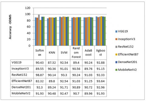
Figure 2 shows the experimental process in effect for the pre-trained CNN models including ResNet-152, VGG-19, DenseNet201, InceptionV3, EfficientNetB7 and MobileNetV2, Figure 4 to Figure 11 evaluate their performance assisted by several classifiers including K-nearest neighbors (KNN), Support Vector Machine (SVM), AdaBoost, Random Forest (RF), Xgboost, and Softmax in the process of classifying tumors in mammography images.
This section compares the Xgboost algorithm with commonly used learning models, such as Random Forest, Adaboost, Support Vector Machine (SVM), K-nearest neighbors (KNN) and CNN, to validate the model. The experiment always uses four measures (F1-Score, Recall, Accuracy and Precision) as the evaluation of the classifier.
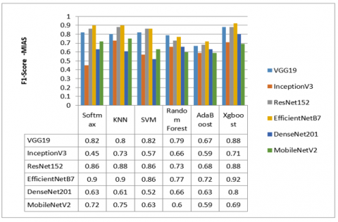
Figure 4 and Figure 5 show the results of the comparison. It was shown that the EfficientNetB7 model combined by the Xgboost classifier outperforms all other pre-trained CNN models among the two datasets (MIAS and DDSM) for all F1-Score values (0.92 for the MIAS dataset and 0.93 for the DDSM dataset). On the other hand, the ResNet-152 model performs very closely to the EfficientNetB7 model. It is observed that the VGG19 model outperforms the EfficientNetB7 model combined with the Random Forest classifier on the MIAS dataset.
It is also shown that the DensNet201 model provides interesting results (0.93) on the DDSM dataset at the same level as the EfficientNetB7 model. This can be explained by the large number of layers in both models.
Figure 4. Results F1-score for MIAS dataset
Figure 5. Results F1-score for DDSM dataset
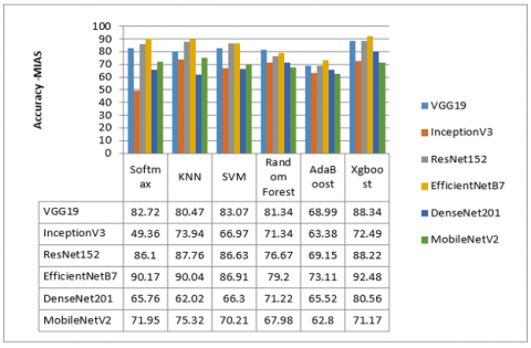
Figure 6. Results accuracy for MIAS dataset
Figure 7. Results accuracy for DDSM dataset
Figure 6 and Figure 7 describe the results of the comparison. It was shown that the EfficientNetB7 model combined with the Xgboost classifier outperforms all other pre-trained CNN models among the two datasets (MIAS and DDSM) for all accuracy values. On the other hand, the ResNet-152 model performs very closely to the EfficientNetB7 model. It is observed that the VGG19 model exceeds the EfficientNetB7 model combined with the Random Forest classifier.
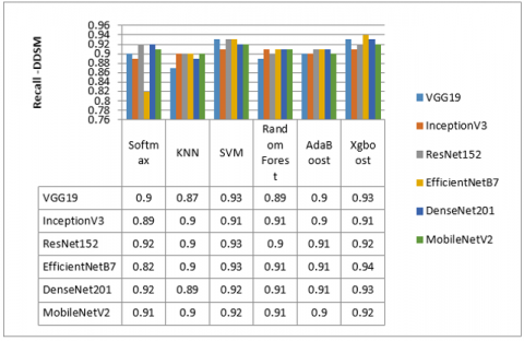
Figure 8 and Figure 9 show the results of the comparison. It was shown that the EfficientNetB7 model combined with the Xgboost classifier outperforms all other pre-trained CNN models among the two datasets (MIAS and DDSM) for all recall values. On the other hand, the ResNet-152 model performs very closely to the EfficientNetB7 model. It is observed that the VGG19 model exceeds the EfficientNetB7 model combined with the Random Forest classifier.
Figure 8. Results recall for MIAS dataset
Figure 9. Results recall for DDSM dataset
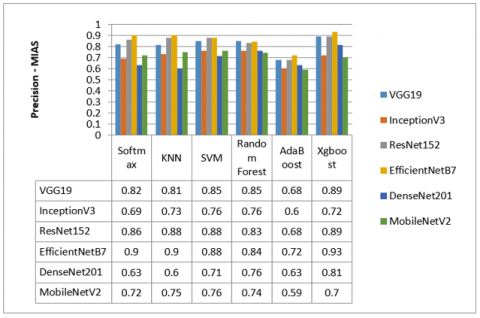
Figure 10. Results precision for DDSM dataset
Figure 11. Results precision for MIAS dataset
Figure 10 and Figure 11 show the comparison results. It was shown that the EfficientNetB7 model combined with the Xgboost classifier outperforms all other pre-trained CNN models among the two datasets (MIAS and DDSM) for all precision values. On the other hand, the ResNet-152 model performs very close to the EfficientNetB7 model. We observe that the ResNet-152 and DenseNet201 models outperform the EfficientNetB7 model combined with the Softmax classifier.
The Xgboost algorithm is the improvement of the Adaboost algorithm and it is confirmed by the results in different CNN architectures. The SVM algorithm performs well with the different CNN models followed by the Xgboost classifier. Indeed, their precision, recall, accuracy and F1-score values are close to those of Random Forest. On the other hand, the Xgboost classifier significantly outperforms the Random Forest algorithm and other classification algorithms with the different CNN models. The interpretation of the results is probably in the fact that it uses the CNN model to automatically extract features that describe the image and less information lost and the acceptable execution time of the Xgboost algorithm to perform the task of classification. These important results demonstrate the effectiveness and efficiency of the novel image classification approach proposed with the CNN-Xgboost model. In fact, EfficientNetB7 has a large number of layers compared to other CNN models. We can state that the Xgboost algorithm performs well with the CNN architecture that the number of layers is large based on the residual.
4.3.2 Case 02: Results of the optimization of the hyper parameters
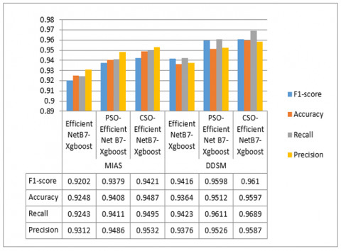
In order to improve the performance of the models, it is performed hyperparameter tuning with the Xgboost classifier. It is showed that the process strongly affected the statistical results with an improvement in most of the four most important measures. The experiment still uses the four measures (F1-Score, Accuracy, Precision and Recall) as the evaluation of the classifier. In this step, the CS algorithm is run with the Xgboost classifier and the CNN EfficientNetB7 model to optimize the four measures.
Figure 12 lists only the important combinations of CS and Xgboost in the case of the EfficientNetB7 model. The process of searching the optimal hyperparameters of the Xgboost classifier showed that a significant improvement was observed when tuning the hyperparameters in the case of the features extracted from the CNN EfficientNetB7 model.
This section defines some parameters with the best performance for experimental comparison and analysis, where eta is 0.33, max_depth is 4, min_child_weight is 0.29, gamma is 0.03, subsample is 0.31 and colsample_tree is 0.14. Next, the EfficientNetB7-CS-Xgboost model is applied to the MIAS and DDSM test sets.
To validate the effectiveness of the EfficientNetB7-CS-Xgboost model, this sub-section compares this model with the EfficientNetB7-PSO-Xgboost and EfficientNetB7-Xgboost models.
Figure 12 shows the variation in the scores of the fourth metric against several combinations of the optimization algorithm and Xgboost in the case of EfficientNetB7. The experimental results demonstrated that EfficientNetB7 (as a feature extractor)+Xgboost (as a classifier)+Cuckoo Search (as an optimizer) is the ideal model for analyzing the mammogram detection task and thus is the custom model presented in this paper.
After performing the above phases to build the model, Figure 12 shows the prediction results of MIAS and DDSM datasets. The parameters of CS were set as follows: number of nests: N=10; nest discovery rate: Pa=0.25; and the maximum number of iterations: tmax=20. To demonstrate the performance of the proposed method, the particle swarm optimization models (EfficientNetB7-PSO-Xgboost) and (EfficientNetB7-Xgboost) were also trained and implemented. The predicted results of these three models were compared and the results of the comparison are shown in Figure 12. The PSO [35] parameters were set as follows: initial population: N=10, local search parameters: C1=1.5; global search parameters: C2=1.7; and maximum number of iterations: tmax=20 and inertia weight (w)=0.8.
Figure 12. Results obtained on the two datasets
Table 5. The optimal hyperparameter for mammography images
|
Parameter |
Interval |
F1-score |
Accuracy |
Recall |
Precision |
|
Eta |
[0,1] |
0.7225 |
0.1826 |
0.6250 |
0.2754 |
|
Min_Child_Weight |
[0,200] |
69 |
45 |
80 |
14 |
|
Max_depth |
[0,200] |
2 |
3 |
0 |
2 |
|
Gamma |
[0,200] |
0.3698 |
0.9894 |
0 |
0.3669 |
|
Subsample |
[0,1] |
0.6568 |
1 |
0.4486 |
0.6545 |
|
Colsample_bytree |
[0,1] |
1 |
0.6899 |
1 |
0.9502 |
Figure 12 shows that the EfficientNetB7-CS-Xgboost model has the highest predictive performance of the both models in both data sets. Although the EfficientNetB7-PSO-Xgboost model has the best prediction performance, the prediction histogram of the EfficientNetB7-CS-Xgboost model is closer to reality than the prediction histogram of the EfficientNetB7-PSO-Xgboost model. The prediction residual of the EfficientNetB7-PSO-Xgboost model is higher than that of the EfficientNetB7-Xgboost model, but its histogram is still relatively small, ranging from 0.01 to 0.10 than that of the EfficientNetB7-CS-Xgboost model. The overall results show that the four-measure error prediction ability of the EfficientNetB7-CS-Xgboost model is better than that of the EfficientNetB7-PSO-Xgboost and EfficientNet-Xgboost models, indicating that CS is an efficient method for hyperparameter optimization among the two data sets.
The optimal hyperparameters for this study are defined in Table 5. This table gives different values of hyperparameters for the optimal results.
Experimental Cases 01 and 02 summarize the results in both cases and perform the above experimental to select the best model for mammography mass lesion classification. In the process of determining the optimal feature extractor among all pre-trained CNN models, EfficientNetB7 performed better than all other models, followed by the Xgboost classifier with the cuckoo search optimization algorithm.
4.4 Discussions
The present study performs the above experimental analysis to select the best model for mammography image classification. The Xgboost classifier is the improvement of the Adaboost algorithm and it is confirmed by the results in different CNN architectures.
In the first stage and according to the experimental results, EfficientNetB7 surpassed all other models with the Xgboost classifier at default values of hyperparameters. Thus, the hyper-parameter optimization process suggested the use of EfficientNetB7 to provide a better feature representation. On the other hand, the Xgboost algorithm significantly outperforms the SVM algorithm and other classifier algorithms with the EfficientNetB7 CNN model. Because it uses CNN to automatically extract good features with less loss of image information and the high speed of Xgboost to achieve efficient classification. These important results confirm the efficiency of the new image classification method proposed with the CNN-Xgboost model. In fact, EfficientNetB7 has a large number of layers compared to other CNN models. Based on experimental results, the Xgboost algorithm performs very well with the CNN model that contains many layers based on the residue. Because Xgboost uses weak basic learning models into a more robust learner in an iterated fashion. At each iteration of gradient boosting, the remaining will be used to adjust the prior predictor to optimize the given loss function. Thus, when the number of CNN layers increases, the number of stronger learners also increases. In fact, the proposed model uses both advantages of the CNN and the Xgboost classifier. The strong advantages of CNN are that it can automatically extract good features and the high advantages of Xgboost classifier are that it can self-correct the weak classifier for previous iterations and use them to build the next tree in the next iteration. The experimental results confirm these two advantages.
In the second stage, while the result of the Xgboost classifier depends largely on the hyper-parameters, it is interesting to optimize these hyper-parameters. Some experiments are conducted with PSO and CS to verify the effectiveness of EfficientNetB7-CS-Xgboost. The experiment always uses the EfficientNetB7 model as the pre-trained CNN model. Figure 12 shows the comparison results and confirms that for both datasets (MIAS and DDSM), both EfficientNetB7-CS-Xgboost and EfficientNetB7-PSO-Xgboost have a better detection effect than EfficientNetB7-Xgboost. On the DDSM and MIAS datasets, the performance difference between EfficientNetB7-CS-Xgboost and EfficientNetB7-PSO-Xgboost is not significant. EfficientNetB7-CS- Xgboost has the best values on all four measures, followed by EfficientNetB7-PSO-Xgboost, which is 1% higher than EfficientNetB7-PSO-Xgboost and 2% higher than EfficientNetB7-Xgboost. The results from these two datasets show that the novel EfficientNetB7-CS-Xgboost approach offers improved prediction performance over the remaining two approaches. This is due to the fact that the CS method discovers the global optimal solution for cases where the search intervals are large and the step distance is small. The control of particle position and velocity in the convergence of the PSO algorithm is too dependent on the current optimal particle, which leads to an early convergence and to the impossibility to find the global optimal solution. Since the CS algorithm uses Lévy's flight search mechanism, it can ignore the local optimal solutions to get the global solution.
4.5 Limitations
Although the results are encouraging, the proposed model still has some limitations that are essential to consider. One of the main limitations of this study is that all revolutionary algorithms have model-dependent parameters, and the actual values/settings of these parameters impact the performance of the algorithm. However, the appropriate setting of the parameters itself becomes an optimization problem. Second, no associated patient history is considered in the proposed evaluation model. Third, while the model uses a large number of convolutional layers, it needs a high computing power; otherwise, it will take a long time in computation.
This research facilitates early diagnosis of mammography to prevent negative impact in these remote areas. The developing of algorithms in this area can be very helpful in achieving better health care services. This paper presents how to use a convolutional neural network with classification algorithms to achieve better medical image identification performance of learning algorithms in the first step, and optimize this new model with the metaheuristic algorithm in the second step. This study observes the performance of different CNN models pre-trained with various classifiers, and then, based on the statistical results, selects the EfficientNetB7 model for the feature extraction step and the Xgboost classifier for classification. Indeed, it is demonstrated that the Xgboost classifier is more suitable for the CNN architecture with a large number of residual layers. The reason is that the Xgboost algorithm performs the weak tree better, which increases the accuracy for each CNN layer. It is more appropriate to combine the CNN architecture that has a low number of layers like VGG-19 and ResNet-50 with the SVM classifier. Nevertheless, it is interesting to achieve the CNN architectures that have many layers like EfficientNetB7 with the Xgboost classifier. In a second step, the CS method is applied with the Xgboost classifier to optimize the hyperparameters. The CS algorithm is applied to choose the appropriate Xgboost parameters to efficiently prevent the phenomenon of "overfitting" or "underfitting" of Xgboost, thus boosting the prediction efficiency. Experiments demonstrate that the proposed model performs well in both datasets. The results of the EfficientNetB7-CS-Xgboost model were compared with those of previous studies, and in particular with the EfficientNetB7-PSO-Xgboost and CNN-Xgboost models over four measures, with the result that the EfficientNetB7-CS-Xgboost model has better accuracy and higher effect than the EfficientNetB7-PSO-Xgboost and EfficientNetB7-Xgboost models. It can be said that this study has improved the efficiency of the model compared to other models (PSO). This novel approach can give, in practice, a novel modeling approach for mammographic tumor classification processing. This model can also be an effective and accurate decision support tool for radiologists and physicians. Nevertheless, the probability parameter in CS is fixed, which can influence the convergence of the algorithm.
The future research direction is to enhance the novel approach in multiple ways, for example by designing an efficient way to improve the performance of the model by optimizing the hyperparameters of EfficientNetB7-CS-Xgboost. Indeed, parameter adjustment is an important area of study [36] that merits more attention. Similarly, a trained convolutional neural network can be integrated with a recurrent neural network (RNN) to improve algorithm performance, while reducing training costs. Finally, combining the Xgboost algorithm with other CNN architectures with a large number of layers can improve classification performance.
[1] Khare, V., Kumari, S. (2022). Performance comparison of three classifiers for fetal health classification based on cardiotocographic data. Acadlore Transactions on AI and Machine Learning, 1(1): 52-60. https://doi.org/10.56578/ataiml010107
[2] Raju, M.S.N., Rao, B.S. (2022). Classification of colon and lung cancer through analysis of histopathology images using deep learning models. Ingénierie des Systèmes d'Information, 27(6): 967-971. https://doi.org/10.18280/isi.270613
[3] Chang, C.C., Lin, C.J. (2011). LIBSVM: A library for support vector machines. ACM Transactions on Intelligent Systems and Technology (TIST), 2(3): 1-27. https://doi.org/10.1145/1961189.1961199
[4] Cover, T., Hart, P. (1967). Nearest neighbor pattern classification. IEEE Transactions on Information Theory, 13(1): 21-27. https://doi.org/10.1109/TIT.1967.1053964
[5] Dasarathy, B.V. (2002). Handbook of data mining and knowledge discovery. Oxford University Press, Inc., New York, NY, USA. Chapter Data Mining Tasks and Methods: Classification: Nearest-Neighbor Approaches, pp. 288-298.
[6] Breiman, L. (2001). Random forests. Machine Learning, 45: 5-32. https://doi.org/10.1023/A:1010933404324
[7] Hastie, T., Rosset, S., Zhu, J., Zou, H. (2009). Multi-class adaboost. Statistics and Its Interface, 2(3): 349-360. https://doi.org/10.4310/SII.2009.v2.n3.a8
[8] Chen, T., Guestrin, C. (2016). Xgboost: A scalable tree boosting system. In Proceedings of the 22nd Acm Sigkdd International Conference on Knowledge Discovery and Data Mining, pp. 785-794. https://doi.org/10.1145/2939672.2939785
[9] Sutskever, K.I.A., Hinton, G.E. (2012). ImageNet classification with deep convolutional neural networks. International Conference on Neural Information Processing Systems Curran Associates Inc., pp. 1097-1105.
[10] Daniel, A.K., Ranjan, R. (2022). An optimized model for sentiment classification using attention oriented hybrid deep learning techniques. International Journal of Artificial Intelligence, 20(01).
[11] Simonyan, K., Zisserman, A. (2014). Very deep convolutional networks for large-scale image recognition. arXiv Preprint, 1409.1556. https://doi.org/10.48550/arXiv.1409.1556
[12] Tan, M., Le, Q. (2019). Efficientnet: Rethinking model scaling for convolutional neural networks. In International Conference on Machine Learning. PMLR, pp. 6105-6114.
[13] Szegedy, C., Vanhoucke, V., Ioffe, S., Shlens, J., Wojna, Z. (2016). Rethinking the inception architecture for computer vision. In Proceedings of the IEEE Conference on Computer Vision and Pattern Recognition, pp. 2818-2826. https://doi.org/10.1109/CVPR.2016.308
[14] He, K., Zhang, X., Ren, S., Sun, J. (2016). Deep residual learning for image recognition. In Proceedings of the IEEE Conference on Computer Vision and Pattern Recognition, pp. 770-778.
[15] Huang, G., Liu, Z., Van Der Maaten, L., Weinberger, K.Q. (2017). Densely connected convolutional networks. In Proceedings of the IEEE Conference on Computer Vision and Pattern Recognition, pp. 4700-4708. https://doi.org/10.1109/CVPR.2017.243
[16] Sandler, M., Howard, A., Zhu, M., Zhmoginov, A., Chen, L.C. (2018). Mobilenetv2: Inverted residuals and linear bottlenecks. In Proceedings of the IEEE Conference on Computer Vision and Pattern Recognition, pp. 4510-4520. https://doi.org/10.48550/arXiv.1801.04381
[17] Jiang, H., He, Z., Ye, G., Zhang, H. (2020). Network intrusion detection based on PSO-XGBoost model. IEEE Access, 8: 58392-58401. https://doi.org/10.1109/ACCESS.2020.2982418
[18] Chen, J., Zhao, F., Sun, Y., Yin, Y. (2020). Improved XGBoost model based on genetic algorithm. International Journal of Computer Applications in Technology, 62(3): 240-245. https://doi.org/10.1504/IJCAT.2020.106571
[19] Wang, H., Yue, W., Wen, S., Xu, X., Haasis, H.D., Su, M., Liu, P., Zhang, S., Du, P. (2022). An improved bearing fault detection strategy based on artificial bee colony algorithm. CAAI Transactions on Intelligence Technology, 7(4): 570-581. https://doi.org/10.1049/cit2.12105
[20] Yang, X.S., Deb, S. (2009). Cuckoo search via Lévy flights. In 2009 World Congress on Nature & Biologically Inspired Computing (NaBIC). IEEE, pp. 210-214. https://doi.org/10.1109/NABIC.2009.5393690
[21] Ker, J., Wang, L., Rao, J., Lim, T. (2017). Deep learning applications in medical image analysis. IEEE Access, 6: 9375-9389. https://doi.org/10.1109/ACCESS.2017.2788044
[22] Varshni, D., Thakral, K., Agarwal, L., Nijhawan, R., Mittal, A. (2019). Pneumonia detection using CNN based feature extraction. In 2019 IEEE International Conference on Electrical, Computer and Communication Technologies (ICECCT), pp. 1-7. https://doi.org/10.1109/ICECCT.2019.8869364
[23] Dubrovina, A., Kisilev, P., Ginsburg, B., Hashoul, S., Kimmel, R. (2018). Computational mammography using deep neural networks. Computer Methods in Biomechanics and Biomedical Engineering: Imaging & Visualization, 6(3): 243-247. https://doi.org/10.1080/21681163.2015.1131197
[24] Arevalo, J., González, F.A., Ramos-Pollán, R., Oliveira, J.L., Lopez, M.A.G. (2015). Convolutional neural networks for mammography mass lesion classification. In 2015 37th Annual International Conference of the IEEE Engineering in Medicine and Biology Society (EMBC), pp. 797-800. https://doi.org/10.1109/EMBC.2015.7318482
[25] Lee, S.J., Chen, T., Yu, L., Lai, C.H. (2018). Image classification based on the boost convolutional neural network. IEEE Access, 6: 12755-12768. https://doi.org/10.1109/ACCESS.2018.2796722
[26] Zhang, X., Nguyen, H., Bui, X.N., Tran, Q.H., Nguyen, D.A., Bui, D.T., Moayedi, H. (2020). Novel soft computing model for predicting blast-induced ground vibration in open-pit mines based on particle swarm optimization and XGBoost. Natural Resources Research, 29: 711-721. https://doi.org/10.1007/s11053-019-09492-7
[27] Jiang, Y., Tong, G., Yin, H., Xiong, N. (2019). A pedestrian detection method based on genetic algorithm for optimize XGBoost training parameters. IEEE Access, 7: 118310-118321. https://doi.org/10.1109/ACCESS.2019.2936454
[28] PUB, M.H., Bowyer, K., Kopans, D., Moore, R., Kegelmeyer, P. (1996). The digital database for screening mammography. In Proceedings of the Third International Workshop on Digital Mammography, Chicago, IL, USA, pp. 9-12.
[29] Sawyer Lee, R., Gimenez, F., Hoogi, A., Rubin, D. (2016). Curated breast imaging subset of DDSM. The Cancer Imaging Archive.
[30] Suckling, J., Parker, J., Dance, D., Astley, S., Hutt, I., (2015). Mammographic image analysis society (MIAS) database v1. 21.
[31] Swathi, K., Kodukula, S. (2022). XGBoost classifier with hyperband optimization for cancer prediction based on geneselection by using machine learning techniques. Revue d'Intelligence Artificielle, 36(5): 665. https://doi.org/10.18280/ria.360502
[32] Eiben, A.E., Smit, S.K. (2011). Parameter tuning for configuring and analyzing evolutionary algorithms. Swarm and Evolutionary Computation, 1(1): 19-31. https://doi.org/10.1016/j.swevo.2011.02.001
[33] Long, W., Liang, X., Huang, Y., Chen, Y. (2014). An effective hybrid cuckoo search algorithm for constrained global optimization. Neural Computing and Applications, 25: 911-926. https://doi.org/10.1007/s00521-014-1577-1
[34] Yang, X.S., Deb, S. (2013). Multiobjective cuckoo search for design optimization. Computers & Operations Research, 40(6): 1616-1624. https://doi.org/10.1016/j.cor.2011.09.026
[35] Challa, R., Rao, K.S. (2021). Hybrid approach for detection of objects from images using fisher vector and PSO based CNN. Ingénierie des Systèmes d'Information, 26(5). https://doi.org/10.18280/isi.260508
[36] Ren, X., Guo, H., Li, S., Wang, S., Li, J. (2017). A novel image classification method with CNN-XGBoost model. In Digital Forensics and Watermarking: 16th International Workshop, IWDW 2017, Magdeburg, Germany, August 23-25, 2017, Springer International Publishing. Proceedings, 16: 378-390. https://doi.org/10.1007/978-3-319-64185-0_28