Lakshmi Tulasi Ravulaplli![]()
© 2023 IIETA. This article is published by IIETA and is licensed under the CC BY 4.0 license (http://creativecommons.org/licenses/by/4.0/).
OPEN ACCESS
Image captioning is the process of creating a textual description of an image. Due to its importance in various fields, it has emerged as the latest and hot research problem. It uses Computer Vision techniques to process an image and Natural Language Processing to generate the caption. Our proposed approach uses the Bi-LSTM (Bi directional Long Short Term Memory) approach to generate the image description. We also propose the Novel Moth Flame Optimization (NMFO). This model uses the correlation-based logarithmic spiral update. The novel proposed model is demonstrated on standard datasets like Flicker 8k, Flicker 30k, and MSCOCO datasets using standard metrics likeBLEU, CIDEr. Performance of various metrics on various datasets shows that our novel Bi-LSTM approach gives better performance when compared to our traditional approaches.
Bi-LSTM, image captioning, inception-v3, NMFO optimization
The general objective domain of Image captioning is to produce English captions to describe images and videos. It is a challenging task. It requires not only object identification, but also the relation among the objects. Image Captioning is important in applications like helping blind people who have the world around, Content-Based image retrieval, bringing visual intelligence to robots, lung cancer detection, web searching, and retrieving images from XML documents. Social networks like Twitter, and Facebook directly generate captions for the images.
Image captioning is easy for humans as it has neurons and its interconnections among them. Initially, this captioning identifies the objects present in the image, their attributes, and the association among the objects, scenes, and scenic locations. Then, it uses the existing templates and grammatical structures to convert the “description data into a sentence with semantics”. But it is a difficult task for machines unless it is trained using better models. The descriptions include where we are and what we wear etc.
In earlier days researchers used basic features like SIFT, HoG, and LBP, and blending of those features is generally used, and features are passed to any one of the classifiers to classify an object. The handcrafted features are task-specific, extracting features from a large and diverse set of data are not feasible.
Deep learning-based algorithms, on the other hand, learn features automatically from training data and can handle massive collections of images and videos. The concerns present in caption generation have emerged as the broader analysis topic in the field of Computer Vision and NLP. Many research works [1-9] proved that deep learning-based approaches can handle the issues raised in image captioning very well. Most of the previous works take the encoder-decoder pattern by using a deep CNN as an encoder to the input image and an additional RNN is used to generate the output caption.
Image captioning is divided into three categories a) Template based b) Retrieval based c) Novelty based. The majority of deep learning-based techniques fall under the area of creating new image captions.
Mao et al. [10] combine visual and textual information using the multimodal layer. But it ignores the intrinsic relations between the predicted words and corresponding visual regions of an image.
An effective proposed approach for image captioning systems must be able to recognize a picture properly while also producing a syntactically valid sentence. The major objective of the image captioning model is to lower the number of classification errors in a sentence composed of several words. To overcome these challenges, we adopt a Bi-LSTM model in this research, in which we deploy a novel optimization approach called the NMFO algorithm to improve the image captioning system's performance. The following are the primary contributions of our study. A novel image caption generator approach is described that extracts features by using the inception v3 model, which is a widely used image recognition model that offers enhanced accuracy on the "Flickr8k dataset” and the “COCO dataset".
For exact image captioning and classification, an Optimized Bi-LSTM model is created, with training taking place under a meta-heuristic model with the suitable tuning of epochs. A novel upgraded logic (logarithmic spiral update based on correlation) is proposed in this research for optimization purposes.
The paper is organized into various sections: In the related work section, a transitory overview of present approaches is discussed. In the proposed model section we describe the novel image caption generation model is elaborated. The methodology followed to carry out our proposed work is discussed. Experimental results discuss the obtained results, Conclusion-The given work is concluded.
We discuss an overview of existing work on LSTM and their domains, as well as alternative approaches, in this section.
Wang et al. [11], have presented a coarse-to-fine strategy that decomposes the original image description into a skeletal statement and the features that go with it. The captioning process is framed in a natural way in this paradigm, with the skeleton phrase being formed first, and then the skeleton's objects being revisited for attribute formation. They ran tests on two datasets, generating descriptive captions with varied lengths for skeleton sentences and attributes independently. They generated the caption in visual space and used the supervised learning approach, whole scene, and encoder-decoder architecture. They have used the ResNet encoder LSTM language model.
Liu et al. [12], have proposed implicit-supervised attention models. Before extracting the feature of the 19-layer VGG net pre-trained on imagenet, resize the considered image to 256 pixels and crop to the 224x224 image at the center. The adam algorithm is used to train the model, which is based on stochastic gradient descent. Regularization is achieved by using dropout. We use the hyperparameters provided in the publicly available code2. They have used 1300 LSTM units while testing with Flickr30k and 1800 LSTM units to test with MSCOCO. They also performed the ground truth attention for a strong supervision model. The Flickr30k entities dataset gives the relevant bounding box of the entity in the image for each entity in the caption. As a result, while predicting the linked words, the model should ideally "attend to" the indicated region. They have limited their evaluation to noun phrases only.
Wu et al. [13], have designed the VQA model which combines the internal representation of the content of an image with the information extracted from the general knowledge base to answer a wide range of image-based questions. To represent the high-level semantic concepts they have used the CNN and RNN approach, further they have used the same mechanism to include external knowledge. They have used the pre-trained VGGNet, LSTM language model on Flickr8k, Flickr30k, and MSCOCO datasets. They have evaluated their model using the BLEU metric.
Zhu et al. [14], two approaches have been devised. The attention model was applied at both the input and output stages of the LSTM to improve sentence creation in the TA-LSTM and PS-LSTM for the picture captioning task. This model successfully creates the picture and makes the words understandable. Finally, CIDEr, BLEU, and ROUGH-L measures were used to evaluate performance. This strategy, however, needs more time to train the model.
Wu et al. [15] have created a novel temporal method for picture captioning that uses g-LSTM to describe the role of visual information at each time period. The visual characteristics were extracted using CNN+RNN. Word-To tackles the word creation problem, word-conditional semantic attention is proposed. Experiments are carried out on typical image captioning benchmarks. The recommended method's success is demonstrated through quantitative and qualitative evaluations.
Huang and Hu [16] have created a c-RNN framework that was created specifically for the captioning process, avoiding word segmentation issues and language tasks in a more efficient manner. The c-RNN also gave the language model access to reason over grammatical rules and word construction in real time, resulting in complex and expressive phrases. Finally, experiments were conducted on the datasets MSCOCO and Flickr30k, demonstrating that c-RNN was capable of faster image prediction.
Karpathy et al. [17], A model basis for a new combination of CNN over image regions and bidirectional (RNN) over phrases presented. Multimodal RNN was used to improve the image resolution. The results were measured using the Flickr8K, Flickr30K, and MS COCO datasets. However, this approach has a computational inefficiency due to the constraint of region assessment in isolation.
The major limitation of RNN, and CNN is that it is difficult to use all visual information for encoding and decoding, which is critical for image caption. The limitation of the LSTM approach is that it uses only the current word (text) to predict the upcoming word and requires more memory space.
To avoid the above-mentioned problems we have designed a model that captures the past and future text simultaneously to achieve high accuracy.
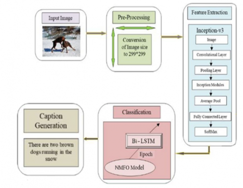
In this section, we discuss the proposed approach for image caption generation in great depth. Figure 1 shows the architectural depiction of the proposed model. The model is comprised of three important phases: “1. Pre-processing, 2. Feature Extraction, 3. Classification”.
Figure 1. The architecture of the proposed model
Irrespective of the dimensions of the input image, we reduce the size of that to 299*299 in the preprocessing phase. Following the pre-processing, feature extraction is to be done using the inception version3 model. Following the extraction of these features, the data is classified by the optimal Bi-LSTM model. The number of epochs of the Bi-LSTM has been tuned in an ideal manner using the NMFO method, which is an improved version of the MFO because the proposed work addresses better image captioning. The implementation is done using the Python language.
3.1 Proposed methodology
Two strategies, Inception-v3 and Bi-LSTM are used in our proposed model. The following sections go through these two in great detail.
3.1.1 Feature extraction of an image
In this phase, we use Inception-v3, which is a traditional deep network made up of eleven modules of five distinct types. Each one of these includes a convolutional layer, an activation layer, a pooling layer, and a batch normalization layer. In this Inception-v3 model [18], these modules are combined to achieve maximum feature extraction. The goal of the Inception-v3 architecture is to use as few computational resources as possible when doing extremely accurate image classification using deep learning. Moreover, it outperforms other deep learning models in terms of caption production [19].
The multi-scale idea is used in the Inception modules. Every module has multiple branches with different kernel sizes, such as "(1x1, 3x3, 5x5, and 7x7)". These filters extract and combine different scales of feature maps, then send the resulting combinations to the next phase. Before deploying "computationally expensive 3x3 and 5x5 convolutions," 1x1 convolutions are used to reduce dimensions in each inception module. The number of Bi-LSTM parameters is reduced by factoring these convolutions into smaller convolutions (3x3). A new set of classification layers is introduced to the datasets in the network graph after the removal of several classification layers and deep inception modules.
3.1.2 Bi-directional LSTM networks
In this phase, we will use the Bi-LSTM network. The features extracted are passed to the Bi-LSTM. This consists of both the forward and backward LSTM layers [20-24]. The framework for the Bi-LSTM is shown in the following Figure 2.
Figure 2. A Bi-LSTM framework for image captioning
The bidirectional technique has been frequently employed in the processing of long sequences since it processes the information from forward and backward directions. A sequence of recurring LSTM cells is included in the LSTM arrangement. The forget gate, the input gate, and the output gate are all represented by three multiplicative units in each LSTM cell. These units allow LSTM memory cells to store and send data for longer periods of time. Let the variables H and C speak for themselves, pointing out the hidden and cell states as needed.
The input and output layers are symbolized by (Xt, Ct-1, Ht-1) and (Ht, Ct) respectively. The process performed by the standard LSTM cell is described below.
The output gate Ot, input gate It, and forget gate Ft correlate to the time phase t in that sequence. The LSTM cell primarily attempts the Ft to filter out information that must be disregarded. The filtered data represents some biased features obtained from a previous frame and connected with the former gaze direction; nonetheless, it should have no effect on the current target. Eq. (1) gives the expression for Ft.
${{F}_{t}}=\sigma \left( {{W}_{IF}}{{X}_{t}}+{{B}_{IF}}+{{W}_{HF}}{{H}_{t-1}}+{{B}_{HF}} \right)$ (1)
In the above equation, (WHF, BHF) and (WIF, BIF) denote the weight matrix and bias parameter that map the hidden layer, and the input layer to the forget gate respectively. The sigmoid function is taken as the gate activation function.
Then, the LSTM cell exploits the input gate for incorporating the suitable information that is given by Eq. (2), Eq. (3), Eq. (4).
${{G}_{t}}=\tanh \left( {{W}_{IG}}{{X}_{t}}+{{B}_{IG}}+{{W}_{HG}}{{H}_{t-1}}+{{B}_{HG}} \right)$ (2)
${{I}_{t}}=\sigma \left( {{W}_{II}}{{X}_{t}}+{{B}_{II}}+{{W}_{HI}}{{H}_{t-1}}+{{B}_{HI}} \right)$ (3)
${{C}_{t}}={{F}_{t}}{{C}_{t-1}}+{{I}_{t}}{{G}_{t}}$ (4)
The above equations, (WHG, BHG) and (WIG, BIG) symbolize the weight matrix and bias parameter that maps the hidden as well as input layers to the cell gate, respectively. The (WHI, BHI) and (WII, BII) correspond to the weight and bias parameter that maps the hidden and input layers to the it respectively.
${{O}_{t}}=\sigma \left( {{W}_{IO}}{{X}_{t}}+{{B}_{IO}}+{{W}_{HO}}{{H}_{t-1}}+{{B}_{HO}} \right)$ (5)
${{H}_{t}}={{O}_{t}}\tanh \left( {{C}_{t}} \right)$ (6)
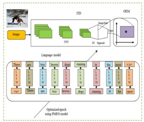
Finally, the LSTM cell achieves the hidden output layer from the output gate, as stated in Eq. (5), Eq. (6), where (WHO, BHO) and (WIO, BIO) are the weight matrix and bias parameter that map the hidden and input layers to Ot respectively. A novel method will be used to optimize the epoch of Bi-LSTM in this project. The framework of an Optimized Bi-LSTM model is shown in Figure 3. The input image, ITD, OEM, and language model make up the architecture. The input pictures are retrieved using CNN in this approach. The Bi-LSTM consists of both the backward and forward LSTM layers that process caption generation in both directions using the NMFO model and an optimal epoch.
Figure 3. Architecture diagram of the proposed Bi-LSTM framework
3.2 The novel MFO algorithm
The traditional MFO technique [25] has a number of advantages, but it also has certain downsides, like local optima, sluggish convergence etc. As a result, various modifications are completed to create a new, optimized model known as the NMFO model to overcome the issues of the previous model. In general, classic optimization techniques have shown that self-improvement is promising [26-31]. The technique for developing a better MFO approach is as follows: This was inspired by their incredible night navigation system. The three most significant phases are included in the MFO.
3.2.1 Initial moths’ population generation
It is considered that all moths move in hyper-dimensional areas. It is represented as in Eq. (7), where the number of moths is written as n and the number of dimensions in solution space is given as d.
$\begin{align} & R=r2;1r2;2\ldots .2;d \\ & rn;1rn;2\ldots rn;d \\ \end{align}$ (7)
Eq. (8) shows the array of the entire moth’s fitness values:
$\mathrm{OR}=\left\{\begin{array}{c}\mathrm{OR} 1 \\ O R 2 \\ \cdot \\ O R n\end{array}\right.$ (8)
Flames and moths are both solutions, with flames being the optimal place for the moth and moths being the genuine search forces that travel about the seeking environment.
3.2.2 Updating the moth’s location
The MFO model is represented as a 3-tuple as shown in Eq. (9).
$M F O=(\operatorname{In}, P, T)$ (9)
In this equation, the initial random position of the moth is shown as ln: $\emptyset \rightarrow\{R, \mathrm{OR}\}$, the movement of the moth in search space is depicted as P: R→R, and the ultimate search process is represented as T: R→{True,False}, lna is a function represented using Eq. (10), which is organized for executing the random distribution.
$R(I,j)=\operatorname{rand}()+lb(i)*(ub(i)-lb(j))$ (10)
In which, the upper and lower boundaries of the variable are denoted ub and lb, respectively. The moth fly employs the traverse orientation in the search space, as explained previously. While employing the logarithmic spiral as a theme, this technique has to deal with three restrictions. The following is a summary of these steps: The NMFO model was used to time the epoch.
1. The spiral's starting point must start with the moth.
2. The flame's location must be the spiral's ultimate point.
3. Spiral range variation must be contained inside the search space.
The proposed contribution is given as follows: The MFO logarithmic spiral is traditionally assessed on the basis of distance and flame. However, as per the new logic, the logarithmic Di=|Uj–Ri| spiral update of MFO takes place based on the correlation factor as shown in Eq. (11). In Eq. (11), CR (Uj, Ri) points out the correlation among Uj and Ri Di is calculated as the average distance of moth ith with jth flame denotes the shape of the logarithmic spiral, and ti is an arbitrary count lies in between -1 and +1.
$S(Ri,Uj)=CR(Uj,Ri)Diebt\cos \left( 2\prod{t}i+Uj \right)$ (11)
3.2.3 Update the flames count
The exploitation phase of the MFO algorithm is enriched by lowering the count of flames. It is computed as per Eq. (12).
flamecount $=\operatorname{round}\left(G-l * \frac{G-l}{G i}\right)$ (12)
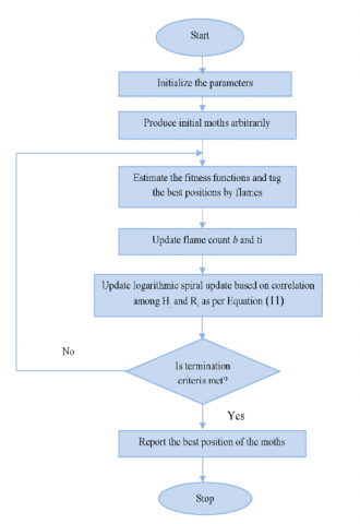
The maximum flame count is shown as G, the iteration count is represented as l, and the maximum iteration count is shown as Gi in Eq. (12). The pseudo-code of the provided NMFO model is shown in the following algorithm, while the flowchart is shown in Figure 4. NMFO begins by randomly creating starting moths within the solution space, then evaluating each moth's fitness function and tagging the optimal position by flame. Then, depending on correlation, update the flame count and the logarithmic spiral update to attain better places marked by a flame. The procedure is repeated until all of the termination requirements have been satisfied.
Figure 4. Flowchart of the NMFO algorithm
NMFO Algorithm
Input: $iter\le {{\max }_{iter}},d,n$
Output: Logarithmic Spiral Update by NMFO
Initiate the Moth flame parameter, position of Moth Ri arbitrarily
For i=1 to n do
Estimate the fitness function Hi
end for
While iter<=max iter
Update the Ri position
Estimate the flame count as per Eq. (12)
Estimate the fitness function Hi
If iter=1
H=sort(R) and OH=sort(OR)
Else
H=sort(Rti-1, Rti) and OH=sort(Rti-1, Rti)
end if
for i=1 to n do
for j=1 to d do
The logarithmic spiral update based on moth value
4.1 Datasets
The “Python” language is used to implement our proposed Bi-LSTM+NMFO scheme for image description generation. Here, we have used two datasets Flickr8k, MSCOCO. The Flickr 8k dataset has a total of 8092 images of different sizes in JPEG format. Out of them, approximately 80% are used for training, 1000 for testing, and the remaining for validation. The COCO dataset is an exceptional object detection dataset that contains 80 classes with 80K, 40K training images, and validation images respectively. Accordingly, the performance of the offered Bi-LSTM+NMFO technique is compared over the other conventional methods like LSTM, c-RNN, Bi-LSTM, and Bi-LSTM+MFO schemes, and the results were observed. For determining the resulting image caption, the BLEU and CIDEr scores were used as caption metrics. In addition, the number of test images used during the analysis varied from 10, 20, 30, 40, 50, and 60.
4.2 Qualitative analysis
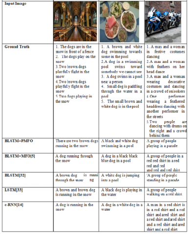
The sample illustration of generated image caption for the Flickr8k dataset is shown in Figure 5. In this analysis quality of our proposed NMFO is compared with the quality of other image captioning techniques such as BLSTM with MFO, BLSTM, LSTM, c-RNN, and deep CNN. Our proposed Bi-LSTM+NMFO approach generated captions very close to the ground truth captions, whereas existing methods like c-RNN, BLSTM, etc. show poor performance compared with other methods.
4.3 Quantitative analysis
Different scores such as BLEU and CIDEr scores are used to assess the quality of the produced caption. The different image captioning approaches were compared here by altering the number of test images. Finally, a performance analysis of the scores has been done for the proposed approach.
Figure 5. The generated caption by various methods for a sample image
4.3.1 Performance analysis using bleu score
The BLEU scores obtained using novel Bi-LSTM+NMFO on the Flicker8k dataset with a varied number of test images (i.e., 25, 50, 75, 100) are shown in Table 1. The obtained scores are better compared with our conventional models like Bi-LSTM with MFO, Bi-LSTM, LSTM, c-RNN, and deep CNN. Similarly, on analyzing the scores, the executed model has attained a higher BLEU score of 0.576685, whereas the score of our conventional models such as BLSTM with MFO, BLSTM, LSTM, c-RNN, and deep CNN has achieved 0.48, 0.553913, 0.452376, 0.233404, and 0.347386 respectively when the test size is 75. Thus, the improvement of the implemented Bi-LSTM+NMFO system has been confirmed from the analysis of results.
The BLEU scores obtained by using the novel Bi-LSTM+NMFO on the MSCOCO dataset with various test sizes (i.e., 25, 50, 75, 100) are shown in Table 2. The attained scores are better compared to our traditional models. When compared to the other models, the provided Bi-LSTM+NMFO model obtained improved score values. When the test size is 100, the implemented strategy achieves a higher BLEU score of 0.813364, whereas traditional models BLSTM with MFO, BLSTM, LSTM, c-RNN, and deep CNN obtained 0.306226, 0.276984, 0.576428, 0.476864, and 0.522186 respectively. The analysis of results, it shows that the Bi-LSTM+NMFO scheme has achieved better results.
Table 1. BLEU score of Bi-LSTM+NMFO over conventional models-Flickr8k dataset
|
Number of test images |
Bi-LSTM+NMFO |
BLSTM with MFO [23] |
BLSTM [2] |
LSTM [24] |
c-RNN [13] |
Deep CNN |
|
25 |
0.607581 |
0.45662 |
0.581667 |
0.615419 |
0.271411 |
0.448415 |
|
50 |
0.608195 |
0.409793 |
0.562438 |
0.501848 |
0.273846 |
0.377847 |
|
75 |
0.576685 |
0.48 |
0.553913 |
0.452376 |
0.233404 |
0.347386 |
|
100 |
0.586482 |
0.417164 |
0.54367 |
0.481175 |
0.252718 |
0.362938 |
Table 2. BLEU score of Bi-LSTM+NMFO over conventional models-MSCOCO dataset
|
Number of test images |
Bi-LSTM+NMFO |
BLSTM with MFO [23] |
BLSTM [2] |
LSTM [24] |
c-RNN [13] |
Deep CNN |
|
25 |
0.761517 |
0.355862 |
0.243973 |
0.475271 |
0.443937 |
0.445109 |
|
50 |
0.773468 |
0.341609 |
0.246418 |
0.562133 |
0.433036 |
0.502536 |
|
75 |
0.796335 |
0.337134 |
0.283871 |
0.591426 |
0.419075 |
0.501801 |
|
100 |
0.813364 |
0.306226 |
0.276984 |
0.576428 |
0.476864 |
0.522186 |
4.3.2 Analysis of cider score
Our proposed Bi-LSTM combined with novel MFO is applied over the traditional models by considering the Flicker8k dataset with respect to the varied number of test images is shown in Table 3. After analysis it is shown that the novel model gives higher CIDEr score compared with the existing models. In almost all the cases our proposed novel approach has achieved higher scores than the traditional approaches except few cases.
On examining the achieved results, the proposed novel model has achieved a better CIDEr score of 0.550779, whereas our conventional models like BLSTM with MFO, LSTM, c-RNN, and Deep CNN have achieved scores of 0.322226, 0.600296, 0.461685, 0.287754, and 0.374725 when the number of images considered for testing is 25. As a result, the achieved outcomes have been used to determine the improvement of the employed Bi-LSTM+NMFO model.
Table 4 shows the CIDEr scores for the MSCOCO dataset achieved by using the new Bi-LSTM+NMFO strategy over traditional models to a variety of test images. After analyzing the results, the given model outperformed the old Model in terms of CIDEr values. On examining the accomplished results, the executed scheme has reached a higher CIDEr score of 0.8377981 whereas, our traditional models such as BLSTM with MFO, LSTM, c-RNN, and deep CNN have achieved minimal CIDEr score of 0.139221, 0.239761, 0.636576, 0.314364, and 0.470214 when the number of images considered for testing is 100. Based on the obtained results, the progress of the employed Bi-LSTM+NMFO model has been established. After analyzing the results, the given model outperformed the old model in terms of CIDEr values. Our proposed approach Bi-LSTM+NMFO is implemented and evaluated on the Flickr8k, and COCO datasets and it gives better performance than the conventional methods. The BLEU and CIDEr scores at the 42nd epoch are mentioned in Table 5.
Table 3. CIDEr score of Bi-LSTM+NMFO over conventional models-flickr8k dataset
|
Number of test images |
Bi-LSTM with NMFO |
BLSTM with MFO [23] |
BLSTM [2] |
LSTM [24] |
c-RNN [13] |
Deep CNN |
|
25 |
0.550779 |
0.322226 |
0.600296 |
0.461685 |
0.287754 |
0.374725 |
|
50 |
0.39951 |
0.234675 |
0.420202 |
0.333022 |
0.166805 |
0.249914 |
|
75 |
0.431215 |
0.214373 |
0.415766 |
0.366305 |
0.163001 |
0.264653 |
|
100 |
0.443517 |
0.213734 |
0.414658 |
0.362103 |
0.162201 |
0.256435 |
Table 4. CIDEr score of Bi-LSTM+NMFO over conventional models-MSCOCO dataset
|
Number of test images |
Bi-LSTM with NMFO |
BLSTM with MFO [23] |
BLSTM [2] |
LSTM [24] |
c-RNN [13] |
Deep CNN |
|
25 |
0.815519 |
0.149880 |
0.261542 |
0.576699 |
0.265719 |
0.421209 |
|
50 |
0.834083 |
0.130739 |
0.236810 |
0.637724 |
0.315885 |
0.476805 |
|
75 |
0.825072 |
0.14027 |
0.247921 |
0.646235 |
0.326357 |
0.467132 |
|
100 |
0.8377981 |
0.139221 |
0.239761 |
0.636576 |
0.314364 |
0.470214 |
Table 5. Proposed model’s performance analysis using bleu, cider on the flickr8k, and MSCOCO datasets
|
Score used |
Epoch number |
Flickr 8k dataset |
MSCOCO dataset |
|
BLEU |
42 |
0.5883 |
0.7988 |
|
CIDEr |
42 |
0.8303 |
0.8341 |
In our work, we introduced a Bi-LSTM-based novel image description generation system that involves three modules, pre-processing of an image, feature extraction of an image, and classification. In the feature extraction phase, we have used the inceptionv3model. Inception-v3 is a popularly used image detection model. Furthermore, an improved Bi-LSTM model was built for exact classification, with the epochs properly calibrated using the NMFO model. Finally, a comparison is done to verify that the proposed technique outperforms previous models.
The BLEU and CIDEr scores are used to assess the quality of the produced caption. The BLEU score and CIDEr score are used to validate the Flicker8k, Flicker30k, and MSCOCO datasets by varying numbers of test images. It is proved that our proposed Bi-LSTM+NMFO outperforms the DCNN, RNN, LSTM, and Bi-LSTM+MFO models. Here, all the results obtained using the currently proposed model i.e., Bi-LSTM+NMFO are higher when compared with the existing models. It shows that our proposed model outperformed the traditional models on the well-known datasets.
[1] Amritkar, C., Jabade, V. (2018). Image caption generation using deep learning technique. In 2018 Fourth International Conference on Computing Communication Control and Automation (ICCUBEA), IEEE, pp. 1-4. https://doi.org/10.1109/ICCUBEA.2018.8697360
[2] Feng, Y., Lapata, M. (2012). Automatic caption generation for news images. IEEE Transactions on Pattern Analysis and Machine Intelligence, 35(4): 797-812. https://doi.org/10.1109/TPAMI.2012.118
[3] Fan, C., Zhang, Z., Crandall, D.J. (2018). Deepdiary: Lifelogging image captioning and summarization. Journal of Visual Communication and Image Representation, 55: 40-55. https://doi.org/10.1016/j.jvcir.2018.05.008
[4] He, X., Yang, Y., Shi, B., Bai, X. (2019). Vd-san: Visual-densely semantic attention network for image caption generation. Neurocomputing, 328: 48-55. https://doi.org/10.1016/j.neucom.2018.02.106
[5] Jamieson, M., Eskin, Y., Fazly, A., Stevenson, S., Dickinson, S.J. (2012). Discovering hierarchical object models from captioned images. Computer Vision and Image Understanding, 116(7): 842-853. https://doi.org/10.1016/j.cviu.2012.03.002
[6] Kahn Jr, C.E., Rubin, D.L. (2009). Automated semantic indexing of figure captions to improve radiology image retrieval. Journal of the American Medical Informatics Association, 16(3): 380-386. https://doi.org/10.1197/jamia.M2945
[7] Liu, Q., Chen, Y., Wang, J., Zhang, S. (2018). Multi-view pedestrian captioning with an attention topic CNN model. Computers in Industry, 97: 47-53. https://doi.org/10.1016/j.compind.2018.01.015
[8] Shetty, R., Tavakoli, H.R., Laaksonen, J. (2018). Image and video captioning with augmented neural architectures. IEEE MultiMedia, 25(2): 34-46. https://doi.org/10.1109/MMUL.2018.112135923
[9] Xu, N., Liu, A.A., Liu, J., Nie, W., Su, Y. (2019). Scene graph captioner: Image captioning based on structural visual representation. Journal of Visual Communication and Image Representation, 58: 477-485. https://doi.org/10.1016/j.jvcir.2018.12.027
[10] Mao, J.H., Xu, W., Yang, Y., Wang, J., Huang, Z.H., Yuille, A. (2014). Deep captioning with multi-modal recurrent neural networks (m-RNN), arXiv:1412: 6632.
[11] Wang, C., Yang, H., Bartz, C., Meinel, C. (2016). Image captioning with deep bidirectional LSTMs. In Proceedings of the 24th ACM International Conference on Multimedia, pp. 988-997. https://doi.org/10.1145/2964284.2964299
[12] Liu, C., Mao, J., Sha, F., Yuille, A. (2017). Attention correctness in neural image captioning. In Proceedings of the AAAI Conference on Artificial Intelligence, 31(1). https://doi.org/10.1609/aaai.v31i1.11197
[13] Wu, Q., Shen, C., Wang, P., Dick, A., Van Den Hengel, A. (2017). Image captioning and visual question answering based on attributes and external knowledge. IEEE Transactions on Pattern Analysis and Machine Intelligence, 40(6): 1367-1381. https://doi.org/10.1109/TPAMI.2017.2708709
[14] Zhu, X.X., Li, L.X., Liu, J., Li, Z.Y., Peng, H.P., Niu, X.X. (2018). Image captioning with triple-attention and stack parallel Lstm. Neurocomputing, 319: 55-65. https://doi.org/10.1016/j.neucom.2018.08.069
[15] Wu, C., Wei, Y., Chu, X., Su, F., Wang, L. (2018). Modeling visual and word-conditional semantic attention for image captioning. Signal Processing: Image Communication, 67: 100-107. https://doi.org/10.1016/j.image.2018.06.002
[16] Huang, G., Hu, H. (2019). C-RNN: A fine-grained language model for image captioning. Neural Processing Letters, 49: 683-691. https://doi.org/10.1007/s11063-018-9836-2
[17] Karpathy, A., Joulin, A., Li, F.F. (2014). Deep fragment embeddings for bidirectional image sentence mapping. Advances in Neural Information Processing Systems, 27. https://doi.org/10.48550/arXiv.1406.5679
[18] Ji, Q., Huang, J., He, W., Sun, Y. (2019). Optimized deep convolutional neural networks for identification of macular diseases from optical coherence tomography images. Algorithms, 12(3): 51. https://doi.org/10.3390/a12030051
[19] Manti, S., Parisi, G.F., Giacchi, V., Sciacca, P., Tardino, L., Cuppari, C., Salpietro, C., Chikermane, A., Leonardi, S. (2019). Pilot study shows right ventricular diastolic function impairment in young children with obstructive respiratory disease. Acta Paediatrica, 108(4): 740-744. https://doi.org/10.1111/apa.14574
[20] Nabati, M., Behrad, A. (2020). Video captioning using boosted and parallel long short-term memory networks. Computer Vision and Image Understanding, 190: 102840. https://doi.org/10.1016/j.cviu.2019.102840
[21] Anuranji, R., Srimathi, H. (2020). A supervised deep convolutional based bidirectional long short term memory video hashing for large scale video retrieval applications. Digital Signal Processing, 102, 102729. https://doi.org/10.1016/j.dsp.2020.102729
[22] Liu, M., Li, L., Hu, H., Guan, W., Tian, J. (2020). Image caption generation with dual attention mechanism. Information Processing & Management, 57(2): 102178. https://doi.org/10.1016/j.ipm.2019.102178
[23] Tan, Y.H., Chan, C.S. (2019). Phrase-based image caption generator with hierarchical LSTM network. Neurocomputing, 333: 86-100. https://doi.org/10.1016/j.neucom.2018.12.026
[24] Zhou, X.L., Lin, J.N., Zhang, Z., Shao, Z.P., Chen, S.Y., Liu, H.H. (2020). Improved itracker combined with bidirectional long short-term memory for 3D gaze estimation using appearance cues. Neurocomputing, 390: 217-225. https://doi.org/10.1016/j.neucom.2019.04.099
[25] Mirjalili, S. (2015). Moth-flame optimization algorithm: A novel nature-inspired heuristic paradigm. Knowledge-Based Systems, 89: 228-249. https://doi.org/10.1016/j.knosys.2015.07.006
[26] Rajakumar, B.R., George, A. (2013). APOGA: An adaptive population pool size-based genetic algorithm. AASRI Procedia, 4: 288-296. https://doi.org/10.1016/j.aasri.2013.10.043
[27] Poluru, R.K., Kumar, R.L. (2019). Enhancement of ATC by optimizing TCSC configuration using adaptive moth flame optimization algorithm. Journal of Computational Mechanics, Power System and Control, 2(3): 1-9. https://doi.org/10.46253/jcmps.v2i3.a1
[28] Rajakumar, B.R. (2013). Static and adaptive mutation techniques for genetic algorithm: A systematic comparative analysis. International Journal of Computational Science and Engineering, 8(2): 180-193. https://doi.org/10.1504/IJCSE.2013.053087
[29] Rajakumar, B.R. (2013). Impact of static and adaptive mutation techniques on the performance of genetic algorithm. International Journal of Hybrid Intelligent Systems, 10(1): 11-22. https://doi.org/10.3233/HIS-120161
[30] Rajakumar, B.R., George, A. (2012). A new adaptive mutation technique for genetic algorithm. IEEE International Conference on Computational Intelligence and Computing Research, pp. 1-7. https://doi.org/10.1109/ICCIC.2012.6510293
[31] Swamy, S.M., Rajakumar, B.R., Valarmathi, I.R. (2013). Design of hybrid wind and photovoltaic power system using opposition-based genetic algorithm with Cauchy mutation. IET Chennai Fourth International Conference on Sustainable Energy and Intelligent Systems (SEISCON 2013), pp. 504-510. https://doi.org/10.1049/ic.2013.0361
[32] Zheng, H., Wu, J.H., Liang, R., Li, Y., Li, X.Z. (2018). Multi-task learning for captioning images with novel words. IET Computer Vision, 13(3): 294-301. https://doi.org/10.1049/iet-cvi.2018.5005
[33] Kinghorn, P., Zhang, L., Shao, L. (2018). A region-based image caption generator with refined descriptions. Neurocomputing, 272: 416-424. https://doi.org/10.1016/j.neucom.2017.07.014