Jakkulla Pradeep Kumar![]() | Ganesh Karthik Muppagowni
| Ganesh Karthik Muppagowni![]() | Jayapal Praveen Kumar
| Jayapal Praveen Kumar![]() | Sree Jagadeesh Malla*
| Sree Jagadeesh Malla*![]() | Suresh Babu Chandanapalli
| Suresh Babu Chandanapalli![]() | Ethala Sandhya
| Ethala Sandhya![]()
© 2023 IIETA. This article is published by IIETA and is licensed under the CC BY 4.0 license (http://creativecommons.org/licenses/by/4.0/).
OPEN ACCESS
Thyroid is on the rise all across the world in modern times. The prevalence of thyroid disease in India is notably high, reaching 1 in 10. Due to the general public's lack of knowledge, the situation with that illness is fast deteriorating. Early diagnosis is crucial so that medical professionals can administer effective treatment before the condition worsens. This is especially true when using deep learning (DL) to predict sickness. One of DL's strengths is its ability to predict how a disease will progress in the future. Once more, several feature selection procedures have benefited in the process of disease prediction and assumption. The most common types of hypothyroidism in this study, we make an effort to predict the initial stage of thyroid development. To achieve this goal, the research has relied heavily on the feature selection strategy in addition to several different categorization methods. Each iteration of the projected adaptive tunicate swarm optimisation (ATSA) consists of two primary phases: searching all over the search space using an arbitrarily picked tunicate and refining the search using the position of the finest tunicate. By making this adjustment, the procedure is better able to explore its environment while simultaneously being protected from the dangers of a sudden convergence. Additionally, a deep convolutional neural network (DeepCNN) is used for disease identification, and the Grey Wolf Optimizer (GWO) is used for its training. Both could be associated more accurately. We were able to improve the suggested model's accuracy to 95% after tweaking the dataset, with 92% specificity.
thyroid disease, adaptive tunicate swarm optimization, Grey Wolf Optimizer, convolutional neural network, hyperthyroid, hypothyroid
The thyroid is the small, butterfly-shaped gland situated near the dishonourable of the neck, just under the skin and muscle. Thyroid glands produce two hormones, levothyroxine (T4) and triiodothyronine (T4). In addition, these glands are vulnerable to a wide range of explicit problems, some of which are more prevalent than others [1]. Hyperthyroidism occurs when the thyroid produces an excessive amount of hormone or too little [2]. The number of nodules has been found inadvertently using TNs detection, which has increased dramatically over the previous few decades [3]. A proper description of nodules could decrease patient risk and therefore minimise it [4]. Most are indolent or benign. As a result, several mathematical models have been used to improve the diagnosis of thyroid nodules. In spite of this, there are obstacles associated with the use of US imaging for sleuthing thyroid nodules [5]. This type of computerised analysis has the potential to improve the interpretation of medical images, allowing for a more trustworthy second opinion to be obtained. such as the liver, breast, and prostate have been the focus of a number of recently introduced software solutions [6]. There are, however, a select few computer-aided diagnostic (CAD) systems available in the United States for evaluating the thyroid. A number of models exist for the automatic detection of variations between normal and inflamed thyroid tissue [7].
To effectively conduct complicated relationship extractions in biomedical information, ML models are progressively being used in the construction of CAD systems [8, 9]. In a similar vein, SVM also plays a crucial role in the diagnosis and staging of thyroid cancer. However, SVM's difficulty lies in its handling of multiclass problems, which increases computing complexity and lengthens training time [10, 11]. Since it is based on the minimization concept of empirical risk, the model-like NN may achieve minima [12]. It is well known that the detection presentation is dependent on the classifier being optimally trained. When the detectors are all the same, however, such as when only images or data are used, the task remains difficult. However, in order to improve clinical diagnostics [13], the use of both data and imaging is required when assessing a thyroid problem. In such a setting, advanced education is mandatory. Although the scenario is becoming increasingly dominated by the deployment of image and data classifiers separately, it is difficult to optimise them for a single goal (label). Both a global classifier that can be used for both the data and the image and a separate enterprise classifier that can be applied to each have been published in the literature [14, 15]. Overfitting and complexity have resulted from their concentration on ad hoc optimisation processes. In this research, we provide a solution to this tricky problem by presenting a global optimisation methodology for dual classifiers.
In order to judge its performance, the suggested method is measured against a number of popular deep learning techniques. There is a 3% improvement in accuracy compared to the baseline DL algorithm. In the following order, the paper is structured: Work relevant to this topic is described in Section 2. The projected algorithm for the model is accessible in Section 3. The projected validation analysis is obtainable in Section 4. In Section 5, we draw some final conclusions and discuss what comes next for this comparative analysis.
Chaganti et al. [16] provide an approach that explores ML/DL models in their publication. A number of different features, including selection, are utilised here. Machine learning-based feature selection is also used, along with extra tree classifiers. Hashimoto's thyroiditis, also known as primary hypothyroidism, increased binding protein, autoimmune thyroiditis, and NTIS, are all conditions that can be predicted using the technique that has been suggested (concurrent non-thyroidal illness). Following extensive research, it was discovered that when combined with the random forest classifier, it produces the best results. These results include a score of F1 and an accuracy of 0.99. The research concluded that when accuracy and the amount of computational effort required were taken into consideration, machine learning models were the most suitable choice for diagnosing thyroid diseases. The k-fold validation and assessment with earlier studies both support the higher presentation of the suggested strategy.
Sankar et al. [17] suggested using the XGBoost algorithm for more precise diagnosis of thyroid conditions. Utilizing the XGBoost feature allows for the selection of the ideal qualities. Methods such as decision trees, regression, and the (KNN) algorithm are utilised in the process of evaluating the proposed XGBoost method. The effectiveness of each of the four distinct algorithms is analysed here, along with their relative strengths and weaknesses. It has been demonstrated that the XGBoost approach has a 2% higher accuracy rate than the KNN algorithm.
For the purpose of classifying thyroid disease, Alsaadawi [18] presents both traditional machine learning models Logistics Regression (LR), and Multi-Layer Perceptron (MLP) and ensemble models (Random Forest (RF), XGBoost, Soft Vote, Stacking, and Bagging). The approach that was suggested went through two stages of training and testing: the first stage utilised all of the features from the dataset, while the second stage utilised only the features that had the highest association, as established by the Recursive Feature Elimination (RFE) model. Despite the fact that DT and MLP both obtained ACCs of 99.92% with all features, MLP was able to attain ACCs of 97.30%, making it the conventional model that was the most accurate. Both the XGboost and the Bagging ensemble models were successful in achieving a flawless ACC. The RFE model, the suggested ensemble models performed significantly better than their baseline equivalents on a range of metrics. An examination of overfitting was carried out on the models that were proposed by using feature selection, cross-validation, and a contrast between the training and test ACC. It was determined that an appropriate amount of time should be devoted to both training and forecasting.
Sureshkumar et al. [19] provide a hybrid optimization selection strategy in order to increase the accuracy of a thyroid disease classifier that uses a rough type-2 fuzzy support vector machine. This was done. This research makes use of a hybrid optimization method, which draws ideas from two different optimization algorithms—the firefly algorithm (FA) and the butterfly optimization algorithm—in order to select the n features that are considered to be the most desirable (BOA). When evaluating the effectiveness of the suggested hybrid firefly butterfly SVM, important parameters such as specificity, accuracy, and sensitivity are taken into consideration (HFBO-RT2FSVM). We compare our approach to industry standards such as the IGWO Linear SVM and the MKSVM, both of which are mixed-kernel adaptations of the support vector machine. Our claim that our method greatly improves accuracy and, as a result, is the gold standard for diagnosing thyroid disease has been supported by experimental investigations and evaluations. The HFBO-RT2FSVM perfect accomplished an accuracy of 99.28% by achieving a specificity of 98% and a sensitivity of 99.2% respectively.
Alyas et al. [20] applied a number of ML procedures, such as decision trees, random forest algorithms, KNN, and artificial neural networks, to the dataset in order to construct a comparative study. The goalmouth of this study was to improve the accuracy with which the disease could be predicted using the parameters recognised from the dataset. In addition, the dataset was altered to achieve a higher degree of accuracy in the classification prediction. Both the sampled and non-sampled datasets were categorised in order to deliver a more precise comparison between the two types of data. After performing various manipulations on the data, we were successful in increasing the accuracy of the random forest method to 94.8 percent, with a specificity of 91.1 percent.
For the purpose of hypothyroidism classification prediction, Guleria et al. [21] utilised a sum of machine learning-based techniques, a (ANN), which is typically used to process text data. These techniques were combined with an ANN-based deep learning (DL) model. The findings of the performance analysis make it abundantly clear that the decision tree and the random forest produce superior results. The accuracy of these two methods is extremely high, coming in at 99.5758% and 99.3107%, respectively, while their error rates are extremely low, coming in at 0.0424 and 0.0689. In addition, we have investigated the precision of the classifiers that have been provided, and we have contrasted the model that has been proposed with models that have been developed in the past; we have found that it is an advancement above the current state of the art. The DL-based ANN model has a high accuracy of 93.8226%, which allows it to compete favourably with other models. In addition, the findings of this research can assist medical professionals in selecting the most appropriate model for diagnosing and classifying hypothyroidism.
The study that was carried out by Zhang et al. [22] makes use of the Xception neural network as its basis and creates a functional background with three different adaptable multi-channel architectures that have been successfully evaluated on data taken from the actual world. The proposed designs were able to attain a diagnosis accuracy degree of 0.989 when using ultrasound images and 0.975 when using scans, respectively, since they made use of a design that had a single input dual-channel configuration. In addition, a patient-specific design was implemented for the purpose of making a diagnosis of thyroid cancer, which resulted architecture, respectively. According to the findings of our research, ultrasonography and computed tomography scans tend to yield diagnostic results that are comparable when utilising computer-aided diagnosis software. The patient-specific analytic design can be reached with CT, while ultrasound images only provide somewhat better results. When making decisions concerning a diagnosis of thyroid cancer, clinicians can utilise the framework that has been proposed to select the architecture that is best appropriate for the situation. The suggested framework also incorporates interpretable results as proof, which has the potential to increase the level of confidence held by medical professionals. This, in turn, may result in a greater adoption of the presented computer-aided diagnosis methods, which are both more accurate and efficient.
This study activity focuses on selecting the most important characteristics and classifying the disease, both of which are detailed in the sections that follow.
3.1 Feature selection technique
The method of feature selection involves automatically selecting those features that are considerably crucial to help in the process of predicting the output or variables that we are interested in. Our dataset contains some inaccurate data, which results in our model having a drastically reduced degree of precision. And in order to get rid of these undesired pieces of data, the technique of feature selection plays a significant part. The advantage of utilising feature selection is because:
3.1.1 Methodology for feature selection
TSA is a straightforward meta that was conceived after observing the behaviour of marine tunicates and the effectiveness of their jet propulsion schemes throughout the processes of navigating and foraging [23]. The size of this animal is measured in millimetres. The tunicate has the ability to find food sources in the water. In spite of this, there is no indication of the food source in the search space that has been provided. When using jet propulsion, a tunicate must fulfil the following as is physically possible. The potential solutions being considered by TSA are on the hunt for the most nutritious food supply. Throughout the course of this procedure, the urochordates will adjust their locations in relation to the best tunicates that will be saved and improved after each cycle. As demonstrated in the following equation, the TSA begins with an inhabitant of tunicates that have been created at random based on the allowable boundaries of the design variables:
$\vec{T}_p=\vec{T}_p^{\min }+\operatorname{rand} \times\left(\vec{T}_p^{\max }-\vec{T}_p^{\min }\right)$ (1)
where, Tp is the location of each urochordate and rand is a random sum between 0 and 1 that falls within the range [0,1]. The lower and upper boundaries of the design variables are denoted by the symbols Tpmin and Tpmax, respectively. The tunicates modify their position according to the following formula [23] while the iterations are taking place:
$\vec{T}_p(\vec{x}+1)=\frac{\vec{T}_p(x)+\vec{T}_p(\vec{x})}{2+c_1}$ (2)
where, c1 is a random sum among zero and one and Tp(x) indicates the tunicate's current location in reference to the food source.
$\vec{T}_p(x)=\left\{\begin{array}{c}S F+A\left|S F-\operatorname{rand} \times \vec{T}_p\right|, \quad \text { if rand } \geq 0.5 \\ S F-A \times \mid S F-\text { rand } \times \vec{T}_p \mid, \quad \text { if rand }<0.5\end{array}\right.$ (3)
where, SF represents the food supply, which is signified by the population's best tunicate location; A denotes a randomised, which is modelled as a probability distribution over all possible combinations of tunicates; and:
$A=\frac{c_2+c_3-2 c_1}{V T_{\min }+c_1\left(V T_{\max }-V T_{\min }\right)}$ (4)
where, c1, c2, and c3 are random values within the range [0; 1]; the least and maximum speeds that are utilised to establish social communication, which are painstaking as 1 and 4, respectively [23]; c1 is the lowest speed and c3 is the highest speed.
The steps of the TSA algorithm are described in the following:
|
Step 1: Initialize the tunicate population TEp based on (1). Step 2: Choose the initial parameters and maximum number of iterations. Step 3: Calculate the fitness value of each search agent. Step 4: The best tunicate is explored in the given search space. Step 5: Update the position of each tunicate using (2). Step 6: Adjust the updated tunicate which goes beyond the boundary in a given search space. Step 7: Compute the updated tunicate fitness value. If there is a better solution than the previous optimal solution, then update the best. Step 8: If the stopping criterion is satisfied, then the algorithm stops. Otherwise, repeat the Steps 5-8. Step 9: Return the best optimal solution which is obtained so far. |
3.1.2 Adaptive tunicate swarm procedure
Even though the TSA can produce efficient results in comparison to other popular procedures, it is not optimal for particularly complicated issues with multiple local optima [24]. Each tunicate in TSA adjusts its position relative to the location of the food source, as demonstrated in Examples (2) and (3). However, if the algorithm reaches premature convergence without any information about the location of the food source (FS), it will be permanently stuck. That is to say, after the algorithm has converged, it is no longer capable of exploring new areas and falls dormant. As a result of this mechanism, the TSA algorithm gets stuck at local minimum points. In light of these constraints, we suggest an adaptable variant of the TSA (ATSA) to address the aforementioned limitations and enhance the algorithm's search capabilities and adaptability.
The search process can be broken down into two parts by a good metaheuristic algorithm: exploration and exploitation. When you explore, you look for new locations far away from where you now are throughout the full search area. The exploration stage involves a metaheuristic algorithm's attempts to catalogue every possible solution and investigate its most promising candidates. However, exploiting is when an optimisation algorithm is able to look for sub-optimal solutions. During this step, the optimizer is able to zero in on the region of the search space that contains the highest-quality solutions. Each time during an iteration of the TSA algorithm, the position of the best solution in the population is updated relative to the other candidate solutions. What this indicates is that the TSA is able to utilise opportunities effectively. Unfortunately, the algorithm's inefficiency in exploring new areas and doing a global search is its Achilles' heel.
The proposed ATSA divides each iteration into two main parts: The exploration phase and the performance phase. Both of these parts are meant to improve the algorithm's ability to perform and explore. In the first stage, called "exploration," the best solution is replaced by a random tunicate, and the order of the tunicates is changed. Also, an optimizer's exploration will be more productive if it uses the randomness that its operators provide. So, the suggested ATSA uses two random integers that are not related to each other in the urochordate's telling equation to make keys for different parts of the search space.
This is a mathematical model of the ATSA's exploration phase:
$\vec{T}_p(\vec{x}+1)=\vec{T}_p(r)-\operatorname{rand}_1 \times\left|\vec{T}_p(r)-2\right| \times \operatorname{rand}_2 \times \vec{T}_p(\vec{x})$ (5)
where, Tp(r) is a sample of the current population of tunicates chosen at random. Each of rand1 and rand2is an arbitrary number between zero and one. In addition to encouraging research, this process strengthens the TSA algorithm's global search across the board.
During the ATSA algorithm's second phase, known as the "exploitation phase," the tunicates adjust their locations to be in line with the best tunicate discovered so far (2). In the projected ATSA, the worst urochordate with the greatest value of the objective function is swapped out for a randomly produced tunicate at each repetition.
Most algorithms' temporal complexity is evaluated by a three-pronged approach. The suggested ATSA's time complexity analysis necessitates similar examination of the following three factors:
First, there is the population initialization time complexity, typically defined as O(ND), where N is the population size and D is the number of dimensions in the problem.
Second, the time difficulty of the first fitness assessment is often measured in terms of O (N F(X)), where F(X) is the impartial function.
Third, the time difficulty of the main loop is typically computed as O (Maxiterations (N D+ N F(X))), where iterations. Thus, the maximum sum of iterations required by the ATSA method is O (Maxiterations (N D+ N F(X))) in order to complete the task.
3.2 Architecture of DeepCNN for classification
This section illustrates the Deep CNN's structural layout. Each of the layers of a Deep CNN to fully Connected (FC) layers. The segmented image is used by the conv layers to create feature maps, which are then sent into the pool layers, the second layer of a Deep CNN. Classification follows the FC layer at long last. Increasing the number of conv layers in Deep CNN improves classification accuracy.
Convolutional layers: The conv layer is employed to create these features and delivers pattern extraction using the object vectors that have been segmented. To generate the feature maps, the inputs are convoluted with the trained weights that are connected to the neurons. To simplify the functional mappings between the input and output variables, the result is then fed into a non-linear activation function. Segmented images produced by the sparking procedure are used as input to the convolution layers in a Deep CNN, and the sum of conv layers is:
$T=\left\{T_1, T_2, \ldots, T_h, \ldots, T_i\right\}$ (6)
Th represents the hth conv layer in Deep CNN, and i represent the total sum of conv layers in Deep CNN. The output, denoted by, is calculated using the input units at (p,w).
$\left(T_v^h\right)_{p, w}=\left(v_v^h\right)_{p, w}+\sum_{p=1}^{w_1^{p-1}} \sum_{z=-r_1^u}^{r_1^u} \sum_{s=-r_2^u}^{r_2^u}\left(X_{f, p}^u\right)_{z, s} *\left(T_v^{h-1}\right)_{p+z, w+s}$ (7)
where, (Xuf,p)(z,s)represents the weights that are skilled using the suggested GWO; * denotes the conv operator that permits the from the yields acquired from the neighbouring conv layers; and W1p-1 represents the total number of feature maps.
Layer of Rectified Linear Units and Pooling (ReLU/POOL): Because of the importance of the ReLU layer in Deep CNN with ReLU, which allows for faster performance when dealing with huge networks, ReLU has become a popular function for assuring efficiency and simplicity. When the ReLU layer is provided with the maps, the resulting output is:
$T_f^u=f u n\left(T_f^{u-1}\right)$ (8)
where, Tfu signifies the input, Tfu-1 signifies the output, and fun() is the activation function for the uth layer.
Completely interconnected layers: The fully layers begin the object classification process with the pattern output from the pooling and conv layers as their input. Completely interconnected layers produce an output that is shown as:
$S_f^u=Z\left(a_f^u\right)$ with $a_f^u=\sum_{p=1}^{w_1^{p-1}} \sum_{m=1}^{w_2^{p-1}} \sum_{n=1}^{w_3^{p-1}}\left(V_{f, p, m, n}^u\right) \cdot\left(T_f^{u-1}\right)_{m, n}$ (9)
The weight between (m,n) in the pth map of layer u-1 and the fth unit in layer u is denoted by V(f,p,m,n)u. The proposed GWO is used to tune the weights appropriately.
3.2.1 Training of DeepCNN
The suggested GWO technique is used to train a DeepCNN classifier for thyroid detection, with the goal of identifying the ideal weights with which to tune the network. The stages taken by the algorithm during the implementation of the proposed GWO procedure are briefly illustrated. To fine-tune the DeepCNN and achieve the best possible classification results, the proposed GWO technique is used to generate the ideal weights. Thyroid detection uses the suggested GWO-based DeepCNN to categorise the input image, coming up with an optimal classification that works well with the influx of new images from dispersed sources. Here are some examples of the algorithmic stages involved in the proposed GWO:
First, we'll do some setup: A solution and its associated parameters are set in motion in the first stage.
$A=\left\{A_1, A_2, \ldots, A_e, \ldots, A_f\right\}$ (10)
The eth solution's location, denoted by Ae, and the total number of solutions, f.
Two, assess the error: Finding the optimal solution requires minimising a fitness function; this is known as the minimization problem, and it is solved by selecting the solution that minimises the Mean Squared Error (MSE). Here is how the MSE is determined.
$M S_{e r r}=\frac{1}{g} \sum_{e=1}^g\left[F_g-F_g^*\right]^2$ (11)
where, Fg is the predictable production and Fg* is the foretold output, g stipulates sum of data samples, where 1<e≤g.
Stage 3: Update weights:
Because the GWO searches for the global optimum rather than settling for a suboptimal solution, it is used to solve practical problems. Grey wolves are used as a model for the GWO algorithm, which mimics their hunting strategy. Wolves' cyclic pattern of hunting behaviour is described in (12-14).
$D=\left|C X_p(t)-X(t)\right|$ (12)
$X(t+1)=X_p-A D$ (13)
In this expression, D is the search distance, A and C are the constants, Xp is the prey's position, t is the repetition number, and X is the wolf's current position. Coefficients A and C are determined using the formulas in (14).
$A=2 a r 1-a, C=2 r 2$ (14)
r1 and r2 are standards fluctuating at random among 0 and 1, as a goes from 2 to 0. Like the wolves' hunting behaviour, described in (15)-(16), the top three solutions are recorded as (16), and (17), and the location is periodically adjusted (18).
$\vec{D}_a=\left|\vec{C}_1 \vec{X}_a-\vec{X}\right|$ (15)
$\vec{D}_\beta=\left|\vec{C}_2 \vec{X}_\beta-\vec{X}\right|$ (16)
$\vec{D}_\delta=\left|\vec{C}_3 \vec{X}_\delta-\vec{X}\right|$ (17)
$\vec{X}(t+1)=\vec{X}_1+\vec{X}_2+\vec{X}_3 / 3$ (18)
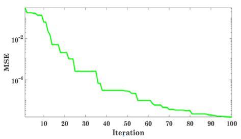
In this case, we have three approximations for distance: X1, X2, and X3, and estimate the location of the prey, while a random location update is made by. The search procedure begins with the development of randomly chosen candidate solutions, which are then refined through a series of iterations in light of the estimated probabilities of where the prey is now located. For the candidate solution to diverge from the true solution or to converge toward it, the conditions A>1 and A1 are required, respectively. After a set number of iterations, the GWO solution from the previous iteration is chosen as the optimal one. In Algorithm I, we outline the procedures that must be carried out in order to achieve optimal settings. Selecting the learning rate is a difficult part of hyper parameter tuning because decreasing it increases the sum of epochs and slows down the process, while increasing it yields a less-than-optimal answer. The suggested method uses the value of the best key found by GWO, which is the step size at which the weights are updated. This is DeepCNN. The objective function of the aforementioned optimizer is to minimise the (MSE) of the MLP. Figure 1 displays the convergence curve between iterations and MSE.
Figure 1. How quickly objective function convergence occurs as a function of iterations
A Core i5 system with 8 GB of RAM and 500 hard discs will run the experiments. Python 3 is the underlying language here. Anaconda and Jupyter Notebook form the basis of the backend. To reap the benefits of being hosted on cloud servers, we are making use of Jupyter Notebook, as indicated in Table 1.
Table 1. Specifications of the proposed model
|
Specifications |
Value |
|
Internet |
8 Mbps download |
|
CPU |
1.5-2.7 GHZ |
|
GPU |
920 m NVidia |
|
RAM |
12 GB |
|
Peers |
4th |
Dataset taken from the UCI data for thyroid illness [20]. The database contains about 7200 different categories of multivariate data. There are 25 distinct characteristics of each record. Out of the total number of variables, 18 are continuous. and 7 are discrete data types as shown in Table 2.
Table 2. Dataset description
|
Dataset characteristics |
Multivariate, field theory |
Sum of instances |
Area |
Life |
7200 |
|
Attribute characteristics |
Definite, real |
Sum of attributes |
Date gave |
1987-01-01 |
25 |
|
Associated tasks |
Organisation |
Missing values? |
Approxi-mately web hits |
254314 |
N/A |
Additionally, to the aforementioned description, the courses are further broken down into the following categories:
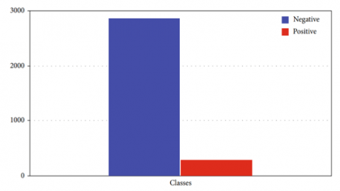
(i) Class-0: negative—2870 trials
(ii) Class-1: positive—293 trials
Figure 2 shows the dataset's missing values, which are denoted by question marks. Take away those additions to lessen the data leakage. By taking this additional measure, the final classification accuracy will improve. From the foregoing, we may assess dataset is skewed with negative incidence than positive. This means that people in class 0 constitute the vast majority. The accuracy of a dataset can be improved through sampling if it is unbalanced. This is done by ensuring that each class is represented equally.
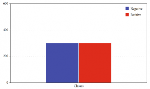
Figure 3 shows that the dataset has been obtained from the UCI dataset repository for thyroid disorders with the intention of using it to train machine learning algorithms. Age, gender, and thyroid indicators are included in the dataset to help classify illness. After analysing the data, we found that only a small percentage of the cases in the dataset are actually positive. TSH, FTI, and T3 readings account for 90% of the classification value since these features contribute more to the dataset on their own, as indicated in Table 3.
Figure 2. Dataset distribution
The suggested algorithm for thyroid illness classification begins with data from the dataset and proceeds through several steps until it finds the best classifier. As can be seen in Figure 3, the dataset was down sampled to make the classes consistent. Since machine learning models are especially vulnerable when faced with skewed data, we normalised the dataset to ensure that our findings are meaningful and not contradictory.
Figure 3. Down tested dataset
Table 3. Dataset attributes
|
Attribute |
Value |
|
Age |
Integer |
|
On thyroxine |
Male (M), female(F) |
|
Query on thyroxine |
(f), (t) |
|
Tumor |
False (f), (t) |
|
Hypopituitary |
False (f), (t) |
|
Pregnant |
False (f), (t) |
|
Query hyperthyroid |
False (f), (t) |
|
Lithium |
False (f), (t) |
|
Goiter |
False (f), t (t) |
|
On antithyroid |
(f), (t) |
|
Sick |
(f), (t) |
|
Psych |
False (f), (t) |
|
TSH measured |
False (f), (t) |
|
T3 measured |
False (f), (t) |
|
T3 |
Real |
|
TT4 measured |
False (f), t (t) |
|
TT4 |
Real |
|
T4U measured |
False (f), true (t) |
|
T4U |
Real |
|
TBG measured |
False (f), true (t) |
|
TBG |
Real |
|
Referral basis |
SVHC, other, SVI, SVHD |
|
Class |
(1), (0) |
4.1 Performances evaluation
Sensitivity, specificity, accuracy, precision, and the F1 score for foretold and annotated outcomes are used to measure the efficacy of the suggested classification setup (19)-(23).
$Accuracy =(T P+T N) /(T P+T N+F P+F N)$ (19)
$Sensitivity =T P /(T P+F N)$ (20)
$Specificity =T N /(T N+F P)$ (21)
$Precision =T P /(T P+F P)$ (22)
$F 1\,\, score =2\left(\frac{\text { Precision } * \text { Recall }}{\text { Precision }+ \text { Recall }} \quad \right)$ (23)
Accuracy describes how well a classifier can make predictions across all three categories (ACC). The percentage of positive examples accurately categorised into one of three groups is the sensitivity (SE). The concept of specificity (SP) focuses on the percentage of false-negatives that are correctly identified. For multiclass issues, precision is a crucial evaluation metric since it indicates the fraction of true positives (TPs) that were correctly identified (relative to the total sum of TPs and Fs). The F1 score incorporates these two metrics as well, since recall indicates the likelihood of false positives when precision does not. It is possible to calculate the total and FN across all three classes by adding the TP, FP, FN, and TN obtained for each class individually. In addition, the classifier efficiency is calculated by applying Eqns. (19)-(23). Results from the performance evaluations and confusion matrices are presented below.
4.2 Performance analysis of the classifiers without feature selection and hyper-parameter tuning (GWO)
In order to confirm the efficiency of projected model, the existing techniques such as XGBoost [17], SVM [18], KNN [18], HFBO-RT2FSVM [19] and ANN [20] are considered. These techniques use various datasets for classification; therefore, all techniques are implemented without considering ATSA and GWO model, then the results are averaged in Table 4.
Table 4. Validation analysis of proposed DeepCNN model
|
Model |
Accuracy |
Recall |
Specificity |
F1-Score |
Precision |
|
XGBoost |
0.83 |
0.85 |
0.91 |
0.89 |
0.89 |
|
SVM |
0.81 |
0.88 |
0.92 |
0.88 |
0.87 |
|
KNN |
0.82 |
0.87 |
0.85 |
0.86 |
0.89 |
|
ANN |
0.86 |
0.89 |
0.89 |
0.85 |
0.90 |
|
HFBO-RT2FSVM |
0.89 |
0.87 |
0.90 |
0.89 |
0.90 |
|
DeepCNN |
0.91 |
0.91 |
0.95 |
0.91 |
0.93 |
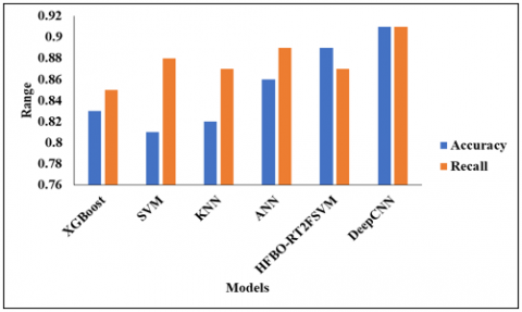
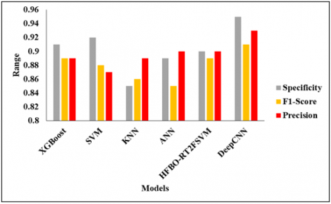
Figure 4. Analysis of projected model without feature selection
Figure 4 represents the analysis of the projected model without the feature selection of different models. Models such as XGBoost, SVM, KNN, ANN, and HFBO-RT2FSVM with DeepCNN. In the analysis of the XGBoost model, the accuracy is 0.83%, and then the SVM model reaches an accuracy of 0.81%. The KNN model reaches an accuracy of 0.82%, and the ANN model reaches an accuracy of 0.86%. Furthermore, the HFBO-RT2FSVMv model reaches an accuracy of 0.89%, and finally, the Deep CNN model reaches an accuracy of 0.91% and a recall value of 0.91%, respectively.
Figure 5. Comparative analysis of DeepCNN without ATSA
Figure 5 represents the comparative analysis of DeepCNN without ATSA. In this analysis, different models. models such as XGBoost, SVM, KNN, ANN, and HFBO-RT2FSVM with DeepCNN. In the analysis of the XGBoost model, the specificity is 0.91%. and then the SVM model reaches an accuracy of 0.92%. The KNN model reaches a specificity of 0.86%, and also the ANN model reaches a specificity of 0.86%. Furthermore, the HFBO-RT2FSVMv model reaches a specificity of 0.90%, and finally, the Deep CNN model reaches a specificity of 0.95%.
4.3 Performance analysis of feature selection techniques (ATSA)
In this section, the proposed ATSA is verified by considering other meta-heuristic models for disease identification. The considered techniques are implemented with our datasets and results are averaged in Table 5.
Table 5. Investigation of projected feature selection techniques
|
Model |
Accuracy |
Recall |
Specificity |
F1-Score |
Precision |
|
GWO |
0.82 |
0.85 |
0.79 |
0.80 |
0.82 |
|
ACO |
0.83 |
0.83 |
0.83 |
0.83 |
0.84 |
|
Firefly |
0.86 |
0.85 |
0.85 |
0.84 |
0.85 |
|
Whale |
0.89 |
0.89 |
0.83 |
0.87 |
0.88 |
|
TSA |
0.91 |
0.91 |
0.87 |
0.91 |
0.91 |
|
ATSA |
0.92 |
0.92 |
0.95 |
0.92 |
0.92 |
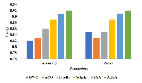
Figure 6. Analysis of projected feature selection model
Figure 6 depicts the Perfect Analysis of Projected Feature Selection. The models such as GWO, ACO, Firefly, Whale, TSA, and ATSA. In the analysis of the GWO model, the accuracy is 0.83%. and then the ACO model reaches an accuracy of 0.83%. The firefly model achieves an accuracy of 0.86%, while the whale model achieves an accuracy of 0.89%. Furthermore, the TSA model achieves an accuracy of 0.91%, while the ATSA model achieves an accuracy of 0.92%.
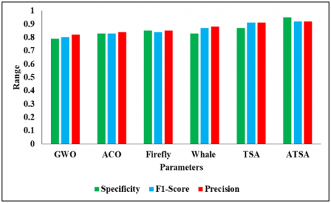
Figure 7. Comparative analysis of ATSA
Figure 7 depicts the Comparative Analysis of ATSA. The models such as GWO, ACO, Firefly, Whale, TSA, and ATSA. In the analysis of the GWO model, the precision is 0.82%. and then the ACO model reaches an accuracy of 0.84%. The whale model has a precision of 0.88%, while the firefly model has a precision of 0.85%. Furthermore, the TSA model reaches the precision of 0.91%, and finally, the ATSA model influences the precision of 0.92% and the f1-score of 0.92%, respectively.
4.4. Performance analysis of proposed model with ATSA and GWO
The existing techniques such as XGBoost [17], SVM [18], KNN [18], HFBO-RT2FSVM [19], and ANN [20] are implemented with GWO. These techniques use various datasets for classification; therefore, all techniques are implemented by considering ATSA, and the results are averaged in Table 6.
Table 6. Validation analysis of proposed model with ATSA and GWO
|
Model |
Accuracy |
Recall |
Specificity |
F1-Score |
Precision |
|
XGBoost |
0.80 |
0.87 |
0.90 |
0.92 |
0.90 |
|
SVM |
0.85 |
0.85 |
0.92 |
0.93 |
0.93 |
|
KNN |
0.87 |
0.87 |
0.84 |
0.87 |
0.88 |
|
ANN |
0.89 |
0.86 |
0.89 |
0.89 |
0.83 |
|
HFBO-RT2FSVM |
0.90 |
0.91 |
0.91 |
0.91 |
0.91 |
|
DeepCNN |
0.96 |
0.94 |
0.96 |
0.94 |
0.95 |
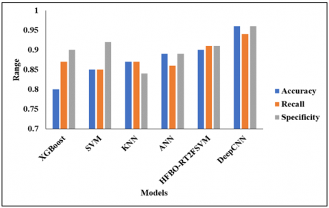
Figure 8. Analysis of proposed model with GWO
Figure 8 depicts the analysis of the proposed model with the GWO model. models such as XGBoost, SVM, KNN, ANN, and HFBO-RT2FSVM with DeepCNN. In the analysis of the XGBoost model, the accuracy is 0.80%. and then the SVM model reaches an accuracy of 0.85%. The KNN model achieves an accuracy of 0.87%, while the ANN model achieves an accuracy of 0.89%. Furthermore, the HFBO-RT2FSVMv model achieves an accuracy of 0.90%, while the Deep CNN model achieves an accuracy of 0.94%.
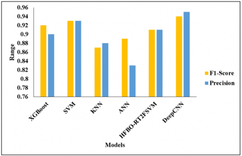
Figure 9. Comparative analysis of ATSA-DeepCNN-GWO
In Figure 9, we represent the comparative analysis of the ATSA-DeepCNN-GWO model. models such as XGBoost, SVM, KNN, ANN, and HFBO-RT2FSVM with DeepCNN. The precision of the XGBoost model in the analysis is 0.90%. and then the SVM model reaches a precision of 0.93%. The KNN model achieves a precision of 0.88%, while the ANN model achieves a precision of 0.83%. Furthermore, the HFBO-RT2FSVMv model reaches a precision of 0.91%, and finally, the Deep CNN model reaches a precision of 0.95% and an F1-score of 0.94%, respectively.
In this study, we present an original technique for detecting thyroid conditions, which entails a two-stage process involving feature selection and classification. The ATSA model is used to pick out the most relevant information from the thyroid dataset. As a result, we also used the DeepCNN model for classification, with GWO performing the hyper-parameter tuning operation. Optimally selecting the DeepCNN convolutional layer was a primary focus of this paper in order to achieve the desired improvement in accuracy. The effectiveness of the proposed ATSO was measured against that of more traditional approaches. The results showed that the proposed model had a 92% accuracy rate and a 95% specificity rate, whereas the existing models only had an 82% to 89% accuracy rate and an 85% to 87.5% specificity rate. The efficacy of the ATSO-DeepCNN-GWO model for thyroid diagnosis was thus demonstrated. We planned to modify Long Term Short Memory (LSTM) algorithms for use with healthcare data in the near future. Therefore, it is more efficient financially and time-wise to design algorithms and thyroid illness prediction models that employ only the most essential criteria for making the diagnosis.
[1] Razia, S., Kumar, P.S., Rao, A.S. (2020). Machine learning techniques for thyroid disease diagnosis: A systematic review. In: Gunjan, V., Zurada, J., Raman, B., Gangadharan, G. (eds) Modern Approaches in Machine Learning and Cognitive Science: A Walkthrough. Studies in Computational Intelligence, vol. 885, Springer, Cham. https://doi.org/10.1007/978-3-030-38445-6_15
[2] Chai, X.Q. (2020). Diagnosis method of thyroid disease combining knowledge graph and deep learning. IEEE Access, 8: 149787-149795. https://doi.org/10.1109/ACCESS.2020.3016676
[3] Vatambeti, R., Mantena, S.V., Kiran, K.V.D., Manohar, M., Manjunath, C. (2023). Twitter sentiment analysis on online food services based on elephant herd optimization with hybrid deep learning technique. Cluster Computing. https://doi.org/10.1007/s10586-023-03970-7
[4] Patra, A., Behera, S.K., Barpanda, N.K., Sethy, P.K. (2022). Effect of microscopy magnification towards grading of breast invasive carcinoma: An experimental analysis on deep learning and traditional machine learning methods. Ingénierie des Systèmes d’Information, 27(4): 591-596. https://doi.org/10.18280/isi.270408
[5] Zhu, Y.C., Al-Zoubi, A., Jassim, S., Jiang, Q., Zhang, Y., Wang, Y.B., Ye, X.D., Du, H.B. (2021). A generic deep learning framework to classify thyroid and breast lesions in ultrasound images. Ultrasonics, 110: 106300. https://doi.org/10.1016/j.ultras.2020.106300
[6] Rao, A.R., Renuka, B.S. (2020). A machine learning approach to predict thyroid disease at early stages of diagnosis. In 2020 IEEE International Conference for Innovation in Technology (INOCON), Bangluru, India, November 06-08, 2020, IEEE, pp. 1-4. https://doi.org/10.1109/INOCON50539.2020.9298252
[7] Halicek, M., Dormer, J.D., Little, J.V., Chen, A.Y., Fei, B. (2020). Tumor detection of the thyroid and salivary glands using hyperspectral imaging and deep learning. Biomedical Optics Express, 11(3): 1383-1400. https://doi.org/10.1364/BOE.381257
[8] Duggal, P., Shukla, S. (2020). Prediction of thyroid disorders using advanced machine learning techniques. In 2020 10th International Conference on Cloud Computing, Data Science & Engineering (Confluence), Noida, India, April 09, 2020, pp. 670-675, IEEE. https://doi.org/10.1109/Confluence47617.2020.9058102
[9] Hosseinzadeh, M., Ahmed, O.H., Ghafour, M.Y., Safara, F., Hama, H.K., Ali, S., Vo, B., Chiang, H.S. (2021). A multiple multilayer perceptron neural network with an adaptive learning algorithm for thyroid disease diagnosis in the internet of medical things. The Journal of Supercomputing, 77: 3616-3637. https://doi.org/10.1007/s11227-020-03404-w
[10] Gao, J., Ismail, N., Gao, Y.J. (2022). Computer big data analysis and predictive maintenance based on deep learning. Ingénierie des Systèmes d’Information, 27(2): 349-355. https://doi.org/10.18280/isi.270220
[11] Peya, Z.J., Chumki, M.K.N., Zaman, K.M. (2021). Predictive analysis for thyroid diseases diagnosis using machine learning. In 2021 International Conference on Science & Contemporary Technologies (ICSCT), Dhaka, Bangladesh, August 05-07, 2021, pp. 1-6, IEEE. https://doi.org/10.1109/ICSCT53883.2021.9642544
[12] Vatambeti, R., Damera, V.K. (2023). Intelligent diagnosis of obstetric diseases using HGS-AOA based extreme learning machine. Acadlore Transactions on AI and Machine Learning, 2(1): 21-32. https://doi.org/10.56578/ataiml020103
[13] Shivastuti, H.K., Manhas, J., Sharma, V. (2021). Performance evaluation of SVM and random forest for the diagnosis of thyroid disorder. International Journal for Research in Applied Science & Engineering Technology, 9: 945-947.
[14] Li, D., Yang, D., Zhang, J., Zhang, X. (2020). Ar-ann: Incorporating association rule mining in artificial neural network for thyroid disease knowledge discovery and diagnosis. IAENG International Journal of Computer Science, 47(1): 25-36.
[15] Bhausaheb, N.R., Vitthal, J.G. (2021). Hybrid classification with meta-heuristic-enabled optimal feature selection for thyroid detection. International Journal of Imaging Systems and Technology. https://doi.org/doi.org/10.1002/ima.22555
[16] Chaganti, R., Rustam, F., De La Torre Díez, I., Mazón, J.L.V., Rodríguez, C.L., Ashraf, I. (2022). Thyroid disease prediction using selective features and machine learning techniques. Cancers, 14(16): 3914. https://doi.org/10.3390/cancers14163914
[17] Sankar, S., Potti, A., Chandrika, G.N., Ramasubbareddy, S. (2022). Thyroid disease prediction using XGBoost algorithms. Journal of Mobile Multimedia, 18: 1-18. http://dx.doi.org/10.13052/jmm1550-4646.18322
[18] Alsaadawi, M.A.W. (2023). Detection of thyroid disease using machine learning models, Karabuk University, Doctoral dissertation.
[19] Sureshkumar, V., Balasubramaniam, S., Ravi, V., Arunachalam, A. (2022). A hybrid optimization algorithm‐based feature selection for thyroid disease classifier with rough type‐2 fuzzy support vector machine. Expert Systems, 39(1): e12811. https://doi.org/10.1111/exsy.12811
[20] Alyas, T., Hamid, M., Alissa, K., Faiz, T., Tabassum, N., Ahmad, A. (2022). Empirical method for thyroid disease classification using a machine learning approach. BioMed Research International. https://doi.org/10.1155/2022/9809932
[21] Guleria, K., Sharma, S., Kumar, S., Tiwari, S. (2022). Early prediction of hypothyroidism and multiclass classification using predictive machine learning and deep learning. Measurement: Sensors, 24: 100482. https://doi.org/10.1016/j.measen.2022.100482
[22] Zhang, X.Y., Lee, V.C.S., Rong, J., Liu, F., Kong, H.Y. (2022). Multi-channel convolutional neural network architectures for thyroid cancer detection. PloS ONE, 17(1): e0262128. https://doi.org/10.1371/journal.pone.0262128
[23] Kaur, S., Awasthi, L.K., Sangal, A.L., Dhiman, G. (2020). Tunicate swarm algorithm: A new bio-inspired based metaheuristic paradigm for global optimization. Engineering Applications of Artificial Intelligence, 90: 103541. https://doi.org/10.1016/j.engappai.2020.103541
[24] Wang, J.Z., Wang, S., Li, Z.W. (2021). Wind speed deterministic forecasting and probabilistic interval forecasting approach based on deep learning, modified tunicate swarm algorithm, and quantile regression. Renewable Energy, 179: 1246-1261. https://doi.org/10.1016/j.renene.2021.07.113