Automatic Detection of Exudates in Retinal Image Using Statistical Techniques

The proposed method of exudates detection is derived into three steps:

• Pre-processing

• Optic disc detection

• Detection of true exudates

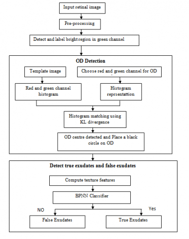
Figure 1 this flow chart shows the algorithm used for the proposed model where it is initially highlighting the pre-processing of the input retinal image that is further deployed for the OD detection so as to identify the false and true exudates from BPNN classifier by computing its texture features generated from OD detection.

1.png

Figure 1. Flow chart of proposed method

2.1 Pre-processing

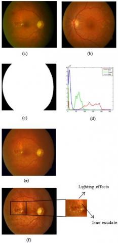
In researches [11, 12] datasets the image available are of different retinal colour, non-uniform illumination and comprising of poor contrast. To deal with these challenges initially few pre-processing steps are essential. In our algorithm pre-processing is divided into three steps as shown in Figure 2 (a-f).

Initially we have removed the non-illumination part at the periphery of retina. For this we have consider red channel of retinal image and perform threshold operation on it using a threshold value [13] typically 35 to generate a binary mask. On this binary mask morphological dilation operation is performed using structural element of disc shape with diameter of 15 pixels. We now apply AND operation of retinal image with resultant mask of eliminated periphery pixels. Secondly to avoid the obstacle of wide variability in colour of retinal images histogram specification operation is used. In histogram specification histogram of test image is reshaped similar to histogram of reference image selected. It leads to similar images in terms of intensity distribution.

2.jpg

Figure 2. (a) Original retinal image; (b) reference image for colour restoration; (c) mask obtained with eliminated periphery pixel; (d) Histogram of reference image; e) Histogram specified image; f) Processed image

Finally, to enhance the contrast of retinal image without affecting its colour information, CIELAB color model is used. CIELAB model decoupled intensity component from colour information (i.e. RGB is converted into ‘L’ ‘A’ ‘B’) where L matrix contains intensity information and A, B matrices contain colour information. Histogram equalization operation is then performed on intensity information ‘L’ matrix while keeping the colour matrix ‘A’ and ‘B’ unchanged. After this test retinal image is again converted into RGB image and used for exudates detection.

As seen, histogram of blue channel is narrow as compared to red and blue channel. Thus green and red channel information is used for exudates detection.

2.2 Count-labelling approach

In count-labelling operation a binary image is obtained corresponds to high intensity pixel in retinal image. The thresholding operation is used to obtain the binary by thresholding the green channel of retinal image with a threshold value ‘T’. But due to non-uniform illumination and lightening effects ‘T’ cannot be a fixed value. The problem of selecting ‘T’ is solved using Otsu algorithm [14] by selecting a local threshold in a block of size 15*15.

2.3 Optic disc detection

Optic disc detection is considered as vital in exudates detection since exudates share similar properties with optic disc in terms of colour, brightness and contrast as seen in Figure 2 (f). It observed that optic disc is a unique region in retinal image having bright pixel and blood vessel converge at it. Thus optic disc can be localized by moving a template of size 80*80 pixels with optic disc at centre at every pixel location in test image. The pixel location with maximum correlation with moving template is said to be location of optic disc. But it is computationally expensive to match 6400 template features at each pixel value in test image. A template of size 80*80 is used to avoid the chances of exudates or noise to be selected as optic disc. In order to reduce the computation cost histogram matching approach using KL divergence approach [15] is used. In histogram matching approach only 512 histogram features are matched (256 histogram feature for red and 256 for green). Secondly in place of matching pixel features at each pixel’s location, only high intensity labelled pixel are considered for OD detection.

Algorithm for OD localization:

1. Input the retinal image and choose its red and green channel for OD detection.

2. Select template image of size 80*80 pixels from training retinal images (typically 3 reference images) with OD at its centre, average them to obtain single template image. Obtain its histogram representation for red and green channel.

3. From test retinal image a window of size 80*80 is chosen across the pixels of higher intensity pixels location labelled above and its red and green channel histogram is computed as shiwn in Figure 3 (a). The histogram of test image is matched with the histogram of reference template using KL divergence approach.

4. In KL divergence method, distance between reference and test histogram is computed as:

Let M and N is probability distribution of occurrence of pixels in test window and reference template window.

$D_{K L}(M / N)_{\text {red }}=\sum_{i=1}^{256} M(i) \log \left(\frac{M(i)}{N(i)}\right)$

$D_{K L}(M / N)_{\text {green }}=\sum_{i=1}^{256} M(i) \log \left(\frac{M(i)}{N(i)}\right)$

$D_{\text {avg }}=\frac{\left|D_{K L}(M / N)_{r e d}\right|+\left|D_{K L}(M / N)_{\text {green }}\right|}{2}$

As we know, KL divergence is a measure of dissimilarity between two distributions. Thus minimum value D_avg leads to maximum correlation and considered as OD location.

3.png

Figure 3. (a) Green channel of test retinal image with localized OD; b) OD excuded retinal image

This OD point obtained is used as seed point and points with maximum intensity are counted. The maximum distance from OD centre to bright pixel is named as radius. Once centre and radius is obtained zero pixel intensity circle is introduced as shown in Figure 3(b).

2.4 Detection of exudates

Exudates detection is divided into two steps:

1. Feature extraction.

2. Classification.

2.4.1 Feature extraction

In this paper for exudates detection, we have considered different existing textural feature extraction technique based on spatial information and compared with proposed one.

(1) GLCM matrix method:

In GLCM [16] the textural features of image are obtained by calculating how often pixel pair occur with specific spatial relationship (i.e. distance and angle) occur in sub region. In this method conditional probability density functions $P(i, j / d, \theta)$ is obtained to estimate the GLCM matrix $\phi(d, \theta)$ as: $\phi_{G L C M}(\mathrm{~d}, \theta)=[P(i, j / d, \theta)], \quad 0<i, j<N_g$.

where, d is inter sample distance, Ɵ is orientation between two pixels and N_g is number of gray level exist in sub-region. In GLCM four different matrixes are considered with different orientation of (0°, 45°, 90°and 135°) are used to represent spatial relationship in all direction. To illustrate the GLCM matrix construction a sample image with eight different gray level is considered as shown in Table 1 and GLCM matrix is obtained with neighbouring distance d=1 and Ɵ=0°, as:

Table 1. GLCM matrix obtained for orientation 0° and neighbouring distance d=1

In GLCM, the limitation is output matrix is always a square matrix of size M*M with entries corresponds to the frequencies of co-occurrence of pixel pairs (where M is corresponding gray level in sub-matrix as shown in Table 2) and does not depend upon the size of input matrix. In GLCM pixel relationship is considered between two pixels. Thus it provides second order textural features. The fine information of exudates can be obtained using higher order textural feature extraction method like GLRLM.

Table 2. Sub image matrix

(2) Gray level run length matrix (GLRLM) method:

The GLRLM [17] matrix method is based on computing run length of gray level (i.e. no of gray level runs exist in sub image of various length). It is computed as how many times a similar pixel is repeated with different length. The GLRLM matrix is represented as shown in Table 3.

$\phi_{G L R L M}(\theta)=[P(i, j / \theta)], \quad 0<i<N_g$ and $0<j \leq R_{\max }$

where, element $P(i, j / \theta)$ is a runlength of gray level ‘i’ of a length ‘j’ (repetition of graylevel ‘i’, ‘j’ times) in the direction $\theta$, N_g is no of gray levels and R_max is no of column in subimage.

Table 3. GLRLM matrix obtained for orientation 0°

In GLRLM method consecutive run of gray level is counted in same row (i.e. P(5,3) represents pixel intensity repeats three times ‘555’ and P(7,2) represent pixel intensity represent ‘77’). Thus it provides higher order feature textural information as compared to GLCM which consider spatial relation of atmost two pixels. In GLRLM matrix column represent the gray level and row represent maximum run of gray level (no of column in sub-matrix) and it depend upon matrix size. But, in GLRLM for computing run length of each gray level we have to traverse the whole sub-matrix every time. Thus it provides high order features (i.e. consider more than two pixels) but it is computationally expensive.

(3) Proposed matrix (GLPCM) method:

In proposed matrix method, we have introduced a higher order feature extraction method with lower computation cost. The idea is to consider the spatial relation between the elements of single row in sub-matrix at one time by counting the occurrence of similar pixels in row. Thus relation between the pixels of complete row is considered by traversing the complete row once and obtained matrix is named as gray level pixel count matrix. The proposed matrix is computed as:

$\phi(\theta)=[P(i, j / \theta)], 0<i<N_g$ and $0<j \leq R_{\max }$

where, $P(i, j / \theta)$ is number of gray level ‘i’ in ‘j’ row of subimage in the direction $\theta$ as shown in Table 4.

Table 4. Proposed matrix $\phi\left(0^{\circ}\right)$ obtained for orientation 0°

The no of rows in proposed matrix is equal no of rows in sub-matrix under consideration and no of column is equal to the no of gray level in sub-matrix. Similarly we can obtained matrix Ø2, Ø3and Ø4 for different orientation of 45° (moving from left diagonal), 90° (vertical direction) and 135° (moving from right diagonal) as shown in Table 5. In proposed matrix method it is not essential that in each case dimension of proposed matrix method is less than GLRLM matrix, but proposed matrix method is less computationally expensive since it consider the count of gray level in one row at a time in place of whole sub matrix. Secondly the obtained matrix can be verified by evaluating the sum of each row which in constant and equal to no of elements in sub matrix.

Table 5. Proposed matrix $\phi\left(90^{\circ}\right)$ obtained for orientation 90°

In this paper we have obtain 6 textural features for each matrices ( $\phi 1, \phi 2, \phi 3$ and $\phi 4$ ). These features are Contrast, Entropy, Energy, Homogeneity, Correlation and dissimilarity as stated [16]. Let $\phi(i, j)$ is a count of pixel ‘i’ in j^th row of sub-matrix locate at position (i,j) in $\phi$ matrix, m is no of rows, n is no of columns and N is the total no of elements in $\phi$ matrix. Then,

Contrast $: \sum_{i=0}^{m-1} \sum_{j=0}^{n-1}\left(|i-j|^2 \varphi(i, j)\right)$

Energy: $\sum_{i=0}^{m-1} \sum_{i=0}^{n-1} \varphi(i, j)^2$

Homogenity: $\sum_{i=0}^{m-1} \sum_{j=0}^{n-1} \frac{\varphi(i, j)}{1+(i-j)^2}$

Entropy: $\sum_{i=0}^{m-1} \sum_{j=0}^{n-1} \varphi(i, j) \log (\varphi(i, j)$

Correlation: $\sum_{\mathrm{i}=0}^{\mathrm{m}-1} \sum_{j=0}^{n-1} \frac{\left(i*j\right) \varphi(i, j)-\mu_x* \mu_y}{\sigma_x* \sigma_y}$

Dissimilarity $: \sum_{i=0}^{g-1} \sum_{j=0}^{g-1}|i-j| p(i, j)$

where,

$\begin{gathered}\mu_x=\frac{1}{N} \sum_{i=0}^{m-1} \sum_{j=0}^{n-1} i \varphi(i, j), \mu_y=\frac{1}{N} \sum_{i=0}^{m-1} \sum_{j=0}^{n-1} j \varphi(i, j) \\ \sigma_x=\sum_{i=0}^{m-1} \sum_{j=0}^{n-1}\left(i-\mu_x\right)^2 \phi(i, j) \\ \sigma_y=\sum_{i=0}^{m-1} \sum_{j=0}^{n-1}\left(j-\mu_y\right)^2 \varphi(i, j)\end{gathered}$

We are considering 6 features for each matrix ( $\phi 1, \phi 2, \phi 3$ and $\phi 4$ ). Thus, we have used 24 features for classification.

2.4.2 Classification

BPNN is a multi-layer feed forward neural network technique based on supervised learning algorithm.in this study two layer neural network is used. The Neural network architecture included an input layer and hidden layer consisting 10 neuron and an output layer comprising of single neuron and tansig function. Following training parameters used: Epochs=1000, Min grad=1e-7, Max fail=6, learning rate=0.01. The network is initially trained using training data for which input and desired output is known. The algorithm modifies the weight on the basis of error back propagation algorithm, so that mean square error (MSE) can be minimized.

Training Phase: BPNN is a supervised learning technique and its accuracy depends upon how well it is trained. In training 20 images are randomly selected contains 15 pathological retinal images and 5 retinal images of healthy patient. Out of these 20 images we have manually selected 1000 pixels and consider a template of size 40*40 around them. These templates comprise of exudates region, optic disc region, blood vessel, normal background and other pathology used to obtain the textural features to train the classifier. In Figure 4, green channel information for different templates images are shown.

4.png

Figure 4. (a) Optic disc region; (b) Blood vessel; (c) Exudates; (d) Normal background

In this study, early stopping is a form of regularization while training a model with an iterative method, such as gradient descent. Since all the neural networks learn exclusively by using gradient descent. Once training phase is complete and optimized value of weights is obtained. We use the same weights for classification between true and false exudates for each test image. Thus, classifier training time is not affecting the entire classification algorithm.

The number of pages for the manuscript must be no more than ten, including all the sections. Please make sure that the whole text ends on an even page. Please do not insert page numbers. Please do not use the Headers or the Footers because they are reserved for the technical editing by editors.