Anandhalekshmi A. Varadharajan*![]() | Srinivasa R. Vaddi
| Srinivasa R. Vaddi![]() | Kanagachidambaresan G. Ramasubramanian
| Kanagachidambaresan G. Ramasubramanian![]()
© 2023 IIETA. This article is published by IIETA and is licensed under the CC BY 4.0 license (http://creativecommons.org/licenses/by/4.0/).
OPEN ACCESS
Internet of Things (IoT) based real-time applications are highly prone to sensor faults because of their deployment in a risky environment. One of the important applications of IoT that is in great demand in this modern era is the air quality monitoring system because of the increase in air pollution over the years around the globe. Hence handling the reliability issue of air quality sensors is of great concern. In this article, a data based diverse fault detection and classification technique is implemented to overcome the sensor fault issue involved in air quality monitoring systems. The proposed work is a two-phase process; first, a Gaussian Hidden Markov Model (GHMM) is used to perform sensor fault detection on real-time air quality sensor data to detect the presence of fault in sensors followed by performing sensor fault classification using a Support Vector Machine (SVM) on the faulty sensor data obtained from fault detection to identify the most difficult to find sensor fault types like ‘Out of bounds’ and ‘Spike fault’. The proposed technique efficiently carries out sensor fault detection and classification with an overall accuracy of 99.48%. Compared to Machine Learning (ML) algorithms like Logistic Regression (LR), Naive Bayes (NB), and Multi-Layer Perceptron (MLP) the diverse proposed technique works well with a precision of 99.50%, recall of 99.08%, and an F1-score of 99.53%.
air quality, fault classification, fault detection, gaussian hidden markov model, internet of things, out of bounds, spike fault, support vector machine
Air pollution is creating a global concern in this modern era because it affects the well-being of humans, ecosystems, etc., around the world. Hence monitoring and analyzing the level of air pollutants around the world holds high priority, for which a portable, cost-effective and efficient air quality monitoring system based on the Internet of Things (IoT) is used. The IoT based monitoring system can effectively detect the air pollutants like carbon monoxide (CO), nitrogen dioxide(NO2), ozone (O3), sulfur dioxide (SO2), particulate matter (PM2.5), methane (CH4) [1], etc., present in the environment through sensors. It can also detect the level of temperature, humidity, and air movements in the environment [2, 3]. It is imperative that the IoT based air quality system must ensure reliability throughout the process because the data from the air quality sensors decide the current condition of the environment [4]. But the sensors involved in the IoT environment are highly prone to faults. The sensor fault includes hard faults and soft faults were in the former fault the sensor nodes could not transfer data to the neighboring or sink node whereas in the latter fault the sensor nodes transfer the faulty data [5]. The soft faults are of serious concern because the user may end up receiving fault data believing it to be normal sensor data leading to false analyses of the air condition. Some of the major sensor fault type includes offset fault, gain fault, stuck-at fault, out of bounds [6], spike fault, noise fault, data loss fault, and random fault [7].
Hence the reliable working of the air quality monitoring system is guaranteed by implementing fault detection and classification on air quality sensor data by applying machine learning (ML) techniques. The ML algorithms can effectively handle and analyze a huge amount of dynamic sensor data [7]. The learning algorithms, based on the provided data grasp pattern automatically, identify complex models and make intelligent decisions. The ML techniques are categorized into three kinds that incorporate supervised learning, unsupervised learning, and semi-supervised learning [8, 9]. Some of the ML algorithms that have accomplished fault detection and classification impactfully on sensor data are k‐Nearest Neighbors (k-NN), Support Vector Machine (SVM) [10], Multi-Layer Perceptron (MLP) [11], Random Forest (RF), and Decision Tree (DT), Neural Network (NN) [12], Principal Component Analysis (PCA), k-means clustering, etc., The evaluation assessment of major ML techniques involved in the air quality monitoring system is done by using the confusion matrix [13]. The efficient analysis of the proposed work is fulfilled using the metrics like precision, recall, F1- score, and accuracy.
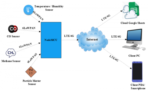
Figure 1 demonstrates the system model of the proposed air quality monitoring system. The air quality sensors used in the monitoring system include a temperature sensor, humidity sensor, carbon monoxide (CO) sensor, methane (CH4) sensor, and particulate matter 2.5 (PM2.5) sensor. The air pollutant data perceived by the air quality sensors are summarized and transmitted using the Node Micro Controller Unit (NodeMCU) via the internet to the client's Personal Computer (PC), Personal Digital Assistant (PDA), smartphone, or the cloud google sheet, from there the necessary data analyzes, aggregation and decision making needed by the client can be done. The protocols used to support the monitoring system for the secure sensor data transmission include ipv6 over Low-Power Wireless Personal Area Networks (6LoWPAN), LTE/4G, etc.
Figure 1. System model of air quality monitoring system
Table 1 denotes the air quality sensor characteristics like connectivity type and data detection limit of sensors like temperature sensor, humidity sensor, CO sensor, CH4 sensor, and PM2.5 sensor considered for the air quality monitoring system.
Table 1. Representing air quality sensor properties
|
Sensors |
Connectivity |
Detecting Range |
|
Temperature sensor |
Digital |
0-50℃ |
|
Humidity sensor |
Digital |
20%-90% |
|
CO sensor |
Analog |
20ppm-2000ppm |
|
CH4 sensor |
Analog |
200ppm-10000ppm |
|
PM2.5sensor |
Analog |
0-1000μg/m3 |
The main contribution of the proposed technique includes,
The remaining section of this article is disbursed as follows: The various fault diagnosis approaches were analyzed in section 2. The proposed diverse technique is defined in section 3. The outcome and analyses of the ML techniques are carried out in section 4. Lastly, section 5 provides an overview of the entire paper.
Wang et al. [14] have described a category-based calibration approach (CCA) for fault tolerance in air quality monitoring sensors. Here the calibration approach uses multiple regression ML techniques like Least Absolute Shrinkage and Selection Operator (LASSO), RF, Extreme Gradient Boosting (XGB), and Light Gradient Boosting Machine (LGBM) to improve the accuracy and robustness of the air quality sensor. The CCA initiates two fault-tolerant modules which include classification tolerance and sample tolerance. The first fault tolerance module reduces the misclassification of sensor data by the regression models and the second module enhances the robustness of unique models. Here the data of carbon monoxide (CO) and Ozone (O3) sensors were considered for the evaluation of CCA. Compared to other machine learning algorithms the LASSO algorithm shows better confidence degree λ=1 using CCA. The Mean Absolute Error (MAE) and Symmetric Mean Absolute Percentage Error (SMAPE) are used to measure the achievements of the suggested approach.
Jan et al. [15] have implemented a distributed sensor-fault detection and diagnosis framework using machine learning for IoT and Cyber Physical Systems (CPS). Here the Stacked Auto- Encoders (SAE) are used to convert the input signal of the Temperature-to-Voltage Converter sensor into a low dimensional feature vector and that is given to the SVM to conduct fault detection. The faulty sensor data from the fault detection block is given as input to the Fuzzy Deep Neural Network (FDNN) of the fault diagnosis block to classify the type of fault like drift, bias, precision degradation, spike, and stuck faults. The working of the framework is assessed based on the metrics like detection accuracy, Area Under the ROC Curve (AUC-ROC), false positive rate, and F1-score. In this paper, the SVM has effectively done fault detection with an accuracy of 99% and the FDNN has executed the fault diagnosis with up to cent percent accuracy.
Saeed et al. [16] have elucidated a machine learning based ensemble technique called extremely randomized trees to carry out fault diagnosis on Wireless Sensor Networks (WSN). Here the extra-tree based diagnostic scheme built different decision trees based on the sensor data and combine those results to effectively detect faults like hard over, drift, spike, erratic, data-loss, stuck, and random fault. Here the dataset considered for the fault diagnosis is the multi-hop networks indoor dataset from which the extremely randomized trees obtain the sensor data as input and detect the faults in the sensors with an accuracy of 81.20%. Compared to the other machine learning algorithms like SVM, RF, MLP, and DT, the explained ensemble learning scheme work better with respect to accuracy, precision, and F1-score.
Lahdhiri et al. [17] have developed an online data-driven fault diagnosis technique for nonlinear industrial process monitoring systems like air quality monitoring systems. Here the sensor fault diagnosis takes place as a two-step process, first online Reduced Rank Optimized Kernel Principal Component Analysis (RR-KPCA) technique is applied for sensor fault detection and next elimination sensor identification (ESI-RRKPCA) is applied for sensor fault isolation. The developed approach is applied to the air quality monitoring network (AIRLOR) where the faults of air quality sensors like Ozone concentration (O3), Nitrogen oxide (NO), and Nitrogen dioxide (NO2) were efficiently detected.
Gupta et al. [18] have implemented a nature-inspired approach called Improved Fault Detection Crow Search Algorithm (IFDCSA) for effectual fault detection in WSNs. Here the real-world datasets considered for detecting sensor faults are intel lab data, multi-hop labeled data and sensorscope data in which the sensor faults are injected based on the crow search algorithm. The fault injected dataset is provided as input to the RF algorithm that successfully classifies sensor faults like stuck‐at fault, drift fault, offset fault, gain fault, noise and spikes. Compared with other machine learning algorithms like RF, k‐NN, DT, and zidi model, the IFDCSA with RF algorithm executes better with an accuracy of 99.94% with very less features.
Mohapatra et al. [19] have explained an improved negative selection algorithm (INSA) with SVM to successfully carry out fault diagnosis in WSN. It is a two-phase process that includes fault detection done by using INSA where the faulty sensor nodes are detected followed by fault classification performed by using multiclass SVM where the type of sensor faults like hard permanent, soft permanent, soft intermittent, and soft transient faults. The assessment metrics considered for this technique are Fault Detection Accuracy (FDA), False Alarm Rate (FAR), False Positive Rate (FPR), Diagnosis Latency (DL), Energy Consumption (EC), Fault Classification Accuracy (FCA), and False Classification Rate (FCR). This technique successfully diagnoses sensor faults in WSN with 99.31% FDA, 4.01% FAR, and 0.69% of FPR.
Zidi et al. [20] have suggested an SVM classification method for the effective detection of sensor faults in WSN. The SVM method efficiently detects faults like offset fault, gain fault, stuck-at fault, out of bounds fault, and random fault. The evaluation metrics considered for this method include Detection Accuracy (DA) and FPR. The SVM method detects faults in sensor networks with an accuracy exceeding 99% and a very less FPR when compared to other techniques like the Hidden Markov Model (HMM), Spatially Organized Distributed Echo State Networks (SODESN), Naive Bayes (NB) classifier and cloud.
3.1 Air quality sensor data
The air quality sensor data that is used for conducting fault detection and classification is the real-time sensor data that is collected over a period using an air quality monitoring system based IoT setup. The sensor data are collected using various air quality sensors like temperature and humidity sensor, CO sensor, CH4 sensor, and dust particle sensor and in the proposed technique the fault detection and classification is done on the data obtained from humidity air quality sensor.
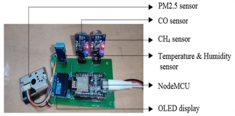
Figure 2 represents the real-time air quality monitoring system setup using nodeMCU. The air quality sensors are connected with nodeMCU through which CO level, CH4 level, dust particle density, temperature, and humidity present in air are stored in the google sheet and in real-time the data are displayed using Organic Light Emitting Diode (OLED) display.
Figure 2. Real-time air quality monitoring system setup using NodeMCU
3.2 Sensor fault detection
The first phase of the proposed diverse technique is fault detection which is done by using the GHMM.
3.2.1 Gaussian hidden markov model
Here the observed humidity sensor data (s1,s2,s3,s4,…..,sn) input that follows gaussian distribution is fed into the GHMM algorithm to carry out fault detection. Here the algorithm predicts the state to which the sensor data input belongs is either “sensor normal” or “sensor faulty” with utmost efficacy. The GHMM for fault detection is represented as follows,
$\left(S_i \mid H_i\right) \sim N\left(\mu_{H_i}, \Sigma_{H_i}\right), i=1,2,3, \ldots n$ (1)
In Eq. (1) Si=(s1,s2,s3,s4,…..,sn) represents the humidity sensor input that follows the normal distribution (N) and Hi=(sn, sf) represents the two hidden states “sensor normal” (sn) and “sensor faulty” (sf) where μHi, ∑Hi represents the mean and covariance parameters at state Hi.
$\lambda=(A, B, \pi)$ (2)
In Eq. (2) A={asn,sf} defines the probability matrix(i.e. the transition probability) of state “sensor normal” (sn) and state“sensor faulty”(sf) and B = {bsn(μi, ∑i, (s1,s2, . . . . sn)) & bsf(μj, ∑j, (s1,s2, . . . . sn))} defines the emission probability parameters of state ‘sn’ and state ‘sf’(i.e. probability that an emitted humidity sensor data become a part of particular state), were μi, ∑i represents the mean and covariance parameter that depends on state ‘sn’ and μj, ∑j represents the mean and covariance parameter that depends on state ‘sf’ and π = {πi} is the initial state distribution. Here the parameters of A and B are iteratively re-estimated for every input sensor data.
Figure 3 depicts a finite state space and homogeneous HMM where the observed distribution of humidity sensor input s1,s2,s3,s4,…..,sn follows the normal distribution. In general, the total transition probability between two states is represented as ‘1’, and the probability that the sensor will move from state ‘sn’ to ‘sf’ is ‘p’ and from ‘sf’ to ‘sn’ is ‘q’. The probability that the sensor will remain in state ‘sn’ is ‘1-p’ and for state ‘sf’ it is ‘1-q’. The state of the sensor is predicted by the HMM as either “sensor normal” (sn) or “sensor faulty” (sf) for every sensor input.
Figure 3. Representing HMM for fault detection
3.3 Sensor fault classification
The second phase of the proposed technique is the fault classification that is accomplished by applying the SVM algorithm [21].
3.3.1 Support vector machine
The SVM classifier technique is a supervised ML algorithm. It takes the output of the fault detection phase as input and performs fault classification effectively. Here the SVM splits the faulty sensor data into two types of fault classes, either as ‘out of bounds’ or as ‘spike fault’ by finding an optimal hyperplane that predicts the fault type with utmost accuracy. The mathematical representation of the hyperplane that do the fault classification is represented using the formula,
$w^T . s_i+b=0$ (3)
In Eq. (3) w is the unit vector representing the normal direction of the decision boundary called the hyperplane and si represents the series of humidity data and b denotes the bias. The support vectors formula for fault prediction is represented as follows,
$h\left(s_i\right)=+1, if w . s+b \geq 0$ (4)
$h\left(s_i\right)=-1, if w . s+b<0$ (5)
Eq. (4) denotes the data points above or on the hyperplane classified as class +1 (i.e., out of bounds) and Eq. (5) denotes the data points below the hyperplane classified as class -1(i.e., spike fault). The decision function of SVM for accurate fault classification is represented using the mathematical expression,
In Eq. (6), si represents the faulty humidity sensor data input vector where the type of sensor fault has to be classified and N indicate the count of support vectors that were acquired prior to the fault classification and the parameters αo,i denotes the best support vector selected for fault prediction.
3.4 Evaluation metrics
The assessment metrics like precision, recall, F1-score, and accuracy are computed based on the confusion matrix in evaluating the performance of the proposed technique. The expressions for the evaluation metrics calculation are represented as follows,
Precision $=\frac{T P}{T P+F P}$ (7)
$\operatorname{Re}$ call $=\frac{T P}{T P+F N}$ (8)
$F 1-$ score $=\frac{2 * \text { precision } * \text { recall }}{\text { precision }+ \text { recall }}$ (9)
Accuracy $=\frac{T P+T N}{T P+F P+T N+F N}$ (10)
From Eqns. (7), (8), (9), and (10) the efficient evaluation of the fault detection and classification technique is done. Here True Positive (TP) indicates the exactly predicted spike faults, True Negative (TN) indicates the exactly predicted out of bounds, False Positive (FP) indicates the falsely predicted out of bounds and False Negative (FN) indicates the falsely predicted spike fault using the confusion matrix.
|
Algorithm 1 Sensor fault detection and classification algorithm. |
|
Input: Real-time humidity sensor data represented as s1, s2, s3, . . . . . . . . . , sn. |
|
Output: Classified sensor fault type as either ‘out of bounds’ or ‘spike fault’. |
|
Procedure: |
|
Step 1: Obtain the humidity sensor data (s1, s2, . . . ., sn) from the real-time air quality monitoring setup. |
|
Step 2: GHMM is employed to conduct the sensor fault detection using the Eqns. (1 & 2). if the humidity data is inside the expected data series limit. then the sensor is “sensor normal”. else the sensor is “sensor faulty”. |
|
Step 3: Execute the sensor fault classification by employing the SVM algorithm using the Eqns. (3-6) to the detected faulty output from step 2. if the faulty humidity data is outside its detection limit. then the sensor fault is “out of bounds”. else if there is a sudden increase in the sensed data than its expected data series. then the sensor fault is the “spike fault”. |
|
Step 4: Result. |
Here in the diverse fault detection and classification technique, both the GHMM and SVM are merged effectively with utmost prediction accuracy.
The real-time air quality data is obtained from the sensors like temperature and humidity sensor, CO sensor, CH4 sensor, and dust particle sensor that were implemented together as an air quality monitoring system setup in a heavy traffic region. Here the fault detection and classification is done on the humidity sensor. The humidity data collected over a period using the air quality monitoring system is injected with 20% of fault data for effective fault diagnosis. Here first sensor data is fed into the GHMM to carry out fault detection followed by achieving fault classification using SVM on the output of GHMM.
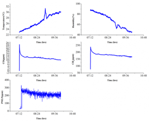
Figure 4 represents air quality data from various sensors like CO sensor, CH4 sensor, PM2.5 sensor, humidity, and temperature sensor collected over a while in a real-time heavy traffic region. The Global Positioning System (GPS) coordinates for the region around which the air quality data were collected are 8°08’47.76” N and 77°19’57.54” E.
Figure 4. Represents sensor data from a real-time air quality monitoring system (8°08’47.76” N & 77°19’57.54” E)
In Figure 5, using the confusion matrix the overall analyses of the implemented sensor fault detection and classification technique is evaluated effectively. The diverse technique executes better with a good accuracy score of 99.48%.
Figure 5. Proposed technique evaluation using confusion matrix
Table 2 depicts the performance comparability of the diverse technique with ML techniques like LR, NB and MLP. Here the proposed work outraces the other techniques with 99.48% accuracy followed by a precision of 99.50%, recall of 99.08% and F1-score of 99.53%.
Table 2. Performance assessment of various ML algorithm
|
Algorithm |
Precision (%) |
Recall (%) |
F1 score (%) |
Accuracy (%) |
|
LR |
63.75 |
43.57 |
51.77 |
54.73 |
|
NB |
76.10 |
78.89 |
77.47 |
74.42 |
|
MLP |
96.56 |
92.20 |
95.94 |
95.65 |
|
GHMM+SVM |
99.50 |
99.08 |
99.53 |
99.48 |
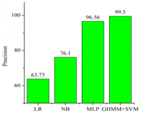
Figure 6 depicts the precision graph comparison of the proposed fault detection and classification technique with algorithms like LR, NB, and MLP. The proposed work executes well with a precision score of 99.50% when compared with the ML algorithms like LR, NB, and MLP whose precision scores are 63.75%, 76.10%, and 96.56%. The proposed diverse technique achieves better precision by 35.75%, 23.4%, and 2.94% than the other ML techniques.
Figure 6. Bar graph for precision comparison
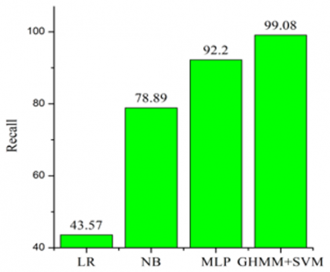
Figure 7 explains the recall graph comparability of the diverse technique with algorithms like LR, NB, and MLP. The proposed work surpassed other algorithms with a recall score of 99.08% than the available ML algorithms whose recall scores are 43.57%, 78.89%, and 92.20%. The proposed fault detection and classification technique excel by 55.51%, 20.19%, and 6.88% than the other ML techniques with respect to recall score.
Figure 7. Bar graph for recall comparison
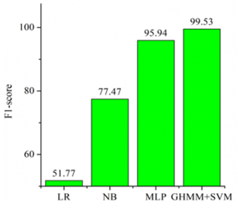
Figure 8 represents the comparison graph of F1-score of the diverse technique with the ML techniques like LR, NB, and MLP. The F1-score is a blend between precision and recall, which ensures an unbiased proposed model in executing the sensor fault detection and classification. The proposed technique accomplishes a better F1-score of 99.53% than the available ML algorithms that have the F1-scores of 51.77%, 77.47%, and 95.94% respectively. The proposed fault detection and classification technique exceed by 47.76%, 22.06%, and 3.59% than the available ML concepts in terms of F1-score.
Figure 8. Bar graph for F1-score comparison
Figure 9 represents the comparison graph for accuracy between the ML concepts like LR, NB, and MLP with that of the proposed diverse sensor fault detection and classification technique. The proposed work is implemented better with an accuracy of 99.48% than the available algorithms and their accuracies are 54.73%, 74.42%, and 95.65%. The proposed technique outraces other ML algorithms by 44.75%, 25.06%, and 3.83% with respect to accuracy.
Figure 9. Bar graph for accuracy comparison
The proposed technique completed sensor fault detection and classification with utmost accuracy thereby reducing the data transfer overhead of the air quality monitoring network by ¼ times in comparison with available ML concepts by communicating only the faulty sensor data to the sink nodes. Thereby the overall performance of the entire air quality network gets enhanced.
In this article, a diverse fault detection and classification technique has been implemented for air quality monitoring systems. Here the proposed task is conducted as a two-phase process, first, the fault detection is executed to identify faulty sensor data using GHMM. In the second phase, fault classification is done by SVM to classify the type of sensor fault. The proposed technique works well with an accuracy of 99.48%. And also evaluation assessment is carried out with the diverse technique and the ML concepts like LR, NB, and MLP based on the performance metrics where the suggested technique achieves a better precision of 99.50%, recall of 99.08%, and F1-score of 99.53%.
Future work of research focus on conducting efficient fault diagnosis on distinct sensor data type and also on more fault types classification involved in air quality monitoring systems.
This experimental task is supported by the Indian Space Research Organization (ISRO) under the research grant reference number No. ISRO/RES/3/843/19-20.
[1] Bajaj, K., Sharma, B., Singh, R. (2020). Integration of WSN with IoT applications: a vision, architecture, and future challenges. Integration of WSN and IoT for Smart Cities, 79-102. https://doi.org/10.1007/978-3-030-38516-3_5
[2] Sampathkumar, A., Murugan, S., Elngar, A.A., Garg, L., Kanmani, R., Malar, A.C.J. (2020). A novel scheme for an IoT-based weather monitoring system using a wireless sensor network. Integration of WSN and IoT for Smart Cities, 181-191. https://doi.org/10.1007/978-3-030-38516-3_10
[3] Xing, L. (2020). Reliability in internet of things: Current status and future perspectives. IEEE Internet of Things Journal, 7(8): 6704-6721. https://doi.org/10.1109/jiot.2020.2993216
[4] Zhang, Z., Mehmood, A., Shu, L., Huo, Z., Zhang, Y., Mukherjee, M. (2018). A survey on fault diagnosis in wireless sensor networks. IEEE Access, 6: 11349-11364. https://doi.org/10.1109/ACCESS.2018.2794519
[5] Kazmi, H.S.Z., Javaid, N., Awais, M., Tahir, M., Shim, S.O., Zikria, Y.B. (2022). Congestion avoidance and fault detection in WSNs using data science techniques. Transactions on Emerging Telecommunications Technologies, 33(3): e3756. https://doi.org/10.1002/ett.3756
[6] Noshad, Z., Javaid, N., Saba, T., Wadud, Z., Saleem, M.Q., Alzahrani, M.E., Sheta, O.E. (2019). Fault detection in wireless sensor networks through the random forest classifier. Sensors, 19(7): 1568. https://doi.org/10.3390/s19071568
[7] Yadav, S.A., Poongodi, T. (2021). A review of ML based fault detection algorithms in WSNs. In: 2021 2nd International Conference on Intelligent Engineering and Management (ICIEM) IEEE, pp: 615-618. https://doi.org/10.1109/ICIEM51511.2021.9445384
[8] Ghosh, N., Maity, K., Paul, R., Maity, S. (2019). Outlier detection in sensor data using machine learning techniques for IoT framework and wireless sensor networks: A brief study. In: 2019 International Conference on Applied Machine Learning (ICAML) IEEE, pp: 187-190. https://doi.org/10.1109/ICAML48257.2019.00043
[9] Azzouz, I., Boussaid, B., Zouinkhi, A., Abdelkrim, M.N. (2020). Multi-faults classification in WSN: A deep learning approach. In: 2020 20th International Conference on Sciences and Techniques of Automatic Control and Computer Engineering (STA) IEEE, pp: 343-348. https://doi.org/10.1109/STA50679.2020.9329325
[10] Javaid, A., Javaid, N., Wadud, Z., Saba, T., Sheta, O.E., Saleem, M.Q., Alzahrani, M.E. (2019). Machine learning algorithms and fault detection for improved belief function based decision fusion in wireless sensor networks. Sensors, 19(6): 1334. https://doi.org/10.3390/s19061334.
[11] Saeed, U., Lee, Y.D., Jan, S.U., Koo, I. (2021). CAFD: context-aware fault diagnostic scheme towards sensor faults utilizing machine learning. Sensors, 21(2): 617. https://doi.org/10.3390/s21020617.
[12] Swain, R.R., Khilar, P.M., Dash, T. (2020). Multifault diagnosis in WSN using a hybrid metaheuristic trained neural network. Digital Communications and Networks, 6(1): 86-100. https://doi.org/10.1016/j.dcan.2018.02.001
[13] Sani, S.H., Shopon, M., Rakib, S.H. (2021). Air quality index prediction using azure IoT machine learning for smart cities. In: Proceedings of International Conference on Computational Intelligence, Data Science and Cloud Computing: IEM-ICDC 2020, pp: 721-733. Singapore: Springer Singapore. https://doi.org/10.1007/978-981-33-4968-1_56
[14] Wang, R., Li, Q., Yu, H., Chen, Z., Zhang, Y., Zhang, L., Zhang, K. (2020). A category-based calibration approach with fault tolerance for air monitoring sensors. IEEE Sensors Journal, 20(18): 10756-10765. https://doi.org/10.1109/jsen.2020.2994645
[15] Jan, S.U., Lee, Y.D., Koo, I.S. (2021). A distributed sensor-fault detection and diagnosis framework using machine learning. Information Sciences, 547: 777-796. https://doi.org/10.1016/j.ins.2020.08.068
[16] Saeed, U., Jan, S.U., Lee, Y.D., Koo, I. (2021). Fault diagnosis based on extremely randomized trees in wireless sensor networks. Reliability Engineering System Safety, 205: 107284. https://doi.org/10.1016/j.ress.2020.107284
[17] Lahdhiri, H., Said, M., Abdellafou, K.B., Taouali, O., Harkat, M.F. (2019). Supervised process monitoring and fault diagnosis based on machine learning methods. The International Journal of Advanced Manufacturing Technology, 102: 2321-2337. https://doi.org/10.1007/s00170-019-03306-z
[18] Gupta, D., Sundaram, S., Rodrigues, J.J., Khanna, A. (2019). An improved fault detection crow search algorithm for wireless sensor network. International Journal of Communication Systems, e4136. https://doi.org/10.1002/dac.4136
[19] Mohapatra, S., Khilar, P.M. (2020). Fault diagnosis in wireless sensor network using negative selection algorithm and support vector machine. Computational Intelligence, 36(3): 1374-1393. https://doi.org/10.1111/coin.12380
[20] Zidi, S., Moulahi, T., Alaya, B. (2017). Fault detection in wireless sensor networks through SVM classifier. IEEE Sensors Journal, 18(1): 340-347. https://doi.org/10.1109/JSEN.2017.2771226
[21] Anandhalekshmi, A.V., Srinivasa, R.V., Kanagachidambaresan, G.R. (2022). Hybrid approach of baum-welch algorithm and SVM for sensor fault diagnosis in healthcare monitoring system. Journal of Intelligent Fuzzy Systems, 42(4): 2979-2988. https://doi.org/10.3233/JIFS-210615