Tao Pan
© 2020 IIETA. This article is published by IIETA and is licensed under the CC BY 4.0 license (http://creativecommons.org/licenses/by/4.0/).
OPEN ACCESS
The feature extraction from athlete action images is a research hotspot. To accurately evaluate athlete actions, it is necessary to partition the original image into refined blocks, and extract different levels of image features. However, the traditional feature extraction algorithms can only roughly divide action images into several classes, failing to acquire the accurate feature sets of the actions. This leads to relatively poor performance of feature extraction from action images. To overcome the defect of the traditional methods, this paper puts forward a feature extraction method for the action images of badminton players based on hierarchical features. The underlying image features were analyzed based on the techniques of badminton players, and mapped to the feature space of the corresponding dimension. Simulation results show that the proposed method can accurately extract the features from athlete action images.
feature extraction, action trajectory, hierarchical features, badminton
In some sports, the athlete needs to do a fixed action after jumping up. This action requires the athlete to have solid skills, and affects the stability of performance [1-3]. To effectively recognize the fixed actions, it is necessary to extract the original features from the action images of the athlete.
Feature extraction from athlete action images has attracted the attention of many scholars [4-10]. For instance, Yi et al. [11] extracted the features from such images through multi-feature fusion and hierarchical backpropagation-adaptive boosting (BP-AdaBoost): a hierarchical recognition framework, including pre-judgment and post-judgment, was adopted to analyze the positions of actions in the images, and divide the images into several classes; then, various features were effectively mined from the images, improving the recognition accuracy of actions. Handri et al. [12] developed a grammar-based feature extraction method for athlete action images. First, every image feature was decomposed into a series of symbols, each of which represents an atomic component of that feature. The atomic components of athlete actions were recognized through intelligent visual analysis, thereby identifying the fixed actions in the images. Zhong et al. [13] designed a multi-temporal feature extraction method for athlete action images: the three-dimensional (3D) direction histogram was employed to compute the points of interest (POIs); the surface and action of the POIs were described by athlete behavioral technology; then, the salient features were extracted from athlete action images.
The development of computer technology has greatly promoted the technical progress of badminton. The tracking and extraction of the action trajectory of badminton players have become a research hotspot [14, 15]. From the perspectives of sports mechanics and badminton sports, experts believe that badminton players rely on the stroking arm to maintain balance, accelerate movements, and increase smash power [16]. Therefore, it is important to track and analyze the trajectory of the stroking actions.
Some methods have already been developed to track the stroking action trajectory of badminton players in action images. Based on hidden Markov model (HMM), Wu et al. [17] proposed a trajectory tracking method for the stroking images of badminton players: Firstly, an HMM was trained with the stroking movements, and the distance between stroking arm targets was calculated in turn; Next, the trajectory features of the stroking actions were subject to dimensionality reduction, followed by fuzzy C-means (FCM) clustering; Finally, the trained HMM was employed to accurately predict the trajectory of the stroking actions. Jiang et al. [18] designed a trajectory tracking strategy for the stroking actions of badminton players based on adaptive threshold segmentation: the stroking arm targets were extracted from the background through adaptive threshold segmentation, using the hexagonal vertebral body model, and used to predict the stroking action trajectory of the target player. With the aid of low angle camera, Zhang et al. [19] presented a trajectory tracking approach for stroking actions of badminton players: First, the 3D information of feature points were acquired from the stroking arm, and the stable and unstable feature points were differentiated by the height of the arm; after that, the stable feature points were tracked, creating the stroking action trajectory.
To sum up, the above trajectory tracking methods can only roughly classify action images into several classes, failing to acquire the accurate feature sets of the actions. This leads to relatively poor performance of feature extraction from action images. To overcome the defect of the traditional methods, this paper puts forward a feature extraction method for the action images of badminton players based on hierarchical features, and evaluates its performance through simulation.
During feature extraction from athlete action images, athlete actions are represented as a consecutive sequence of states. Each state has its own dynamic features. Traditionally, the local features are extracted from each image. Then, the local features of all images are divided into multiple grids in time and space. From the spatial and temporal distributions of local features, the overall features of athlete action images can be derived. Mathematically, the feature extraction process can be described as follows:
Let $(x, y, t, \sigma, \tau)$ be the consecutive sequence of states, where $(x, y, t)$ are the dynamic features of each action. The overall features of athlete action images can be derived from the spatial and temporal distributions of local features in multiple grids:
$H=\frac{\operatorname{det}(\mu)-{ktrace}^{3}(\mu)}{(x, y, t, \sigma, \tau) \times(x, y, t)}$ (1)
where, $\mu$ and k are the spatial and temporal meshing of the local features, respectively; trace $^{3}$ is the distribution of the athlete action images.
Nevertheless, the traditional method merely divides athlete action images into rough classes, without generating accurate feature sets of the actions. In this case, it is impossible to extract high-quality features from action images.
To track the stroking action trajectory of badminton players, the two-dimensional (2D) coordinates and velocity of each action were identified through image processing and matching. Then, the recursive relationship between stroking arm targets was calculated. After that, a Kalman filter state estimation model was established based on the relationship and minimum variance estimation, and used to predict the stroking action trajectory. Mathematically, the trajectory tracking process can be illustrated as:
Let $\left(x_{k-1}, y_{k-1}\right)$ and respectively be the coordinates of an action in time k-1 and time k, respectively; $\left(v_{x}, v_{y}\right)$ be the stroking velocity; t be the sampling period. Then, the recursive relationship between stroking arm targets can be expressed as:
$\left\{\begin{array}{l}x_{k}=x_{k-1}+t v_{x} \\ y_{k}=y_{k-1}+t v_{y}\end{array}\right.$ (2)
Then, the Kalman filter state estimation model can be established as:
$x_{k}^{\prime}=A x_{k-1}+B$ (3)
where, $x_{k}^{\prime}$ is the state vector of stroking actions; A is the state transition matrix of stroking actions; B is the input matrix. The error covariance of trajectory prediction can be calculated by:
$p_{k}^{\prime}=A P_{k-1} A Q_{k-1}$ (4)
where, $p_{k}^{\prime}$ and $P_{k-1}$ are the error covariance matrices of $x_{k}^{\prime}$ and $x_{k-1}$, respectively; $Q_{k-1}$ is the state correction equation for the trajectory prediction. The x-axis coordinate of an action in time k can be expressed as:
$x_{k}=x_{k}^{\prime}+K_{k}\left(z_{k}-H_{k} x_{k}^{\prime}\right)$ (5)
where, $z_{k}$ is the observation vector of stroking actions; $H_{k}$ is the system observation matrix. Then, image matching was implemented to determine the coordinates and velocity of stroking actions. The coordinates of each action can be expressed as $z_{k}=\left(x w_{k}, y w_{k}, x v_{k}, y v_{k}\right)^{T}$. Eq. (6) is used to give the Kalman filter gain coefficient $K_{k}$ of correcting section.
$K_{k}=p_{k}^{\prime} H_{k}\left(H_{k} p_{k}^{\prime} H_{k}+R_{k}\right)^{-1}$ (6)
where, $P_{k}$ is the covariance matrix of the observation noise in time k; $w_{k}$ and $v_{k}$ are vectors of independent zero-mean Gaussian white noise. Then, the covariance correction equation can be established as:
$P_{k}=\left(I-K_{k} H_{k}\right) p_{k}^{\prime}$ (7)
where, $P_{k}$ is the error covariance correction matrix in time k; I is the identity matrix.
3.1 Potential function of action sequence
To optimize the extraction of hierarchical features from athlete action images, the Harris 3D operator was introduced to mine the most salient points in time and space from the fixed action frames in each original image. The features of each salient point were obtained from the gradient histogram and the streamer direction histogram, denoted as 2D and 90D, respectively. Together, the features of each salient point were expressed as a 162D eigenvector, which serves as a low-level feature of athlete action images.
Then, the coordinates of each salient point of the body were obtained from the original image. Here, the coordinates $\left(x_{z i}, y_{z i}\right)$ of the 20 most salient points are used, and seven local centers $\left(a_{i}, b_{i}\right)$ are selected from the body: head, two arms, two legs, and two feet. The distance from every salient point $\left(x_{j}, y_{j}\right)$ to each center can be calculated by:
$n=\frac{\arg\underrightarrow{\min } }{\left(x_{z i}, y_{z i}\right)} \sqrt{\left(a_{i}-x_{i}\right)^{2}+\left(b_{i}-y_{i}\right)^{2}}$ (8)
The distance defines the range of the salient point in time and space. Thus, all the salient points of the action images could be divided into 7 parts, $n=1, \ldots, 7$. The seven parts of salient points were categorized into 3 levels:
High level: the salient points on this level reflect the details about the coordinates and action features;
Middle level: the salient points on this level roughly reflect the coordinates and action features;
Low level: the salient points on this level only reflect the action features.
After the categorization, the low-level features were subject to k-means clustering (KMC). The KMC outputs a K*162D image of 3 levels and 7 parts, based on the number of cluster heads. In each part, the T consecutive frames of each fixed action were defined as the spatiotemporal unit of the action. The unit represents the action features of the corresponding body part in a period. Two units are connected by T/2 overlapping frames. Then, all the spatiotemporal units in each action image were merged into a sequence of units.
The bag-of-words (BOW) feature in the n-th range of the p-th image in the action image set can be expressed as:
$f_{p}=\frac{K_{n} \times n}{K} \times \frac{(K \times 162)}{p}$ (9)
where, N is the length of the sequence of units; $K_{n}$ is the number of cluster heads in the n-th range.
By the BOW feature of each image, the features of each part were fused preliminarily by:
$F_{P}=\sum_{n \in\{1,7\}} K_{n} \times N$ (10)
where, $F_{P}$ is the fused feature of each part on the corresponding level of each image.
After preliminary fusion, the action image sequence and sequence tag were denoted as $X=\left\{X_{i}\right\}_{i=1}^{t}$ and Y, respectively. From formula (10), the conditional probability of athlete action images can be modeled as:
$P(Y, h \mid X, \theta)=\left\{X_{i}\right\}_{i=1}^{t} \times F_{p} \times \frac{\exp \left(f_{p} \cdot \varphi(Y, h, X)\right)}{\sum\left(F_{P} \cdot \varphi\left(Y^{\prime}, h, X\right)\right)} F_{P}$ (11)
where, $\varphi(Y, h, X) \in \zeta$ is the potential function of action sequence.
According to the features of action changes, the potential of action changes on each level in the action image sequence can be derived from formula (11) as:
$\varphi(Y, h, X)=\left(\sum_{j \in v} \varphi_{1}\left(X_{j}, h_{j}\right), \sum_{j \in v} \varphi_{2}\left(Y, h_{j}\right)\right) \frac{\sum_{(j, k) \epsilon \varepsilon} \varphi_{3}\left(Y, h_{j}, h_{k}\right)}{P(Y, h \mid X, \theta)}$ (12)
where, $\varphi_{1}\left(X_{j}, h_{j}\right)$ is the relationship between prediction nodes and hidden variable nodes; $\varphi_{2}\left(Y, h_{j}\right)$ is the relationship between hidden variable nodes and the tagged points of the action image sequence; $\varphi_{3}\left(Y, h_{j}, h_{k}\right)$ is the relationship between hidden variable nodes and the tagged points, i.e. the relationship between action migration and action difference.
If $h_{j}$ satisfies the condition that the node corresponding to the hidden state of athlete action images in class Y of fixed actions, the potential function equals 1; otherwise, the potential function equals 0. If the primitive actions of $h_{j}$ to $h_{k}$ conform to the process of action Y, the potential function equals 1; otherwise, the potential function equals 0.
3.2 Feature extraction
The above subsection set up the potential function of the action image sequence for different levels of action changes. Here, the AdaBoost algorithm is introduced to screen the features that contribute the most to the analysis of athlete action images, and take them as the training and test samples. The specific steps are as follows:
Let $\left(x_{1}, y_{1}\right), \cdots\left(x_{i}, y_{i}\right), \cdots\left(x_{N}, y_{N}\right)$ be the training set of athlete action images, where $x_{i}$ is an athlete action image, $y_{i}$ is the tag of the image, and N is the total number of training images. During the training, some training images were randomly selected as unknown samples. Then, the AdaBoost algorithm was implemented as a weak classifier to get the hypothesis condition $h_{t}\left(x_{i}\right) \in\{1,-1\}$ of each training image. Based on $\varphi(Y, h, X)$, the error rate of all athlete action images can be calculated by:
$\varepsilon_{t}=\frac{\varphi(Y, h, X) \times\left(h_{t}\left(x_{i}\right) \neq y_{i}\right)}{\left(x_{1}, y_{1}\right), \cdots\left(x_{i}, y_{i}\right), \cdots\left(x_{N}, y_{N}\right)}$ (13)
According to the result of formula (13), the class of athlete action to be extracted from the N training images was tagged as 1, and the other classes were tagged as -1. Then, random parts were selected iteratively, forming the training samples, and the nearest neighbor classifier was used as a weak classifier. On this basis, the feature extraction model was established as:
$\widehat{C_{l}}=\operatorname{agr} \min _{C}\left\|d_{i}-C\left(d_{j}\right)^{2}\right\| \times \varepsilon_{t}$ (14)
where, $d_{i}$ is the i-th feature in the test set; $C\left(d_{j}\right)$ is the class of the j-th action feature in the training image; $\varepsilon_{t}$ is the relative deviation in the training process.
4.1 Detection of moving targets
To begin with, the differential calculation was implemented to obtain the stroking action image sequence of two consecutive frames. Then, a Gaussian model was constructed for the grayscale distribution of the difference image. After that, the expectation maximization (EM) algorithm was adopted to estimate the Gaussian model parameters of the difference image. Thereafter, the boundary detection operator was introduced to construct the boundary image, such as to extract the contour of moving targets in the stroking process. Mathematically, the specific process can be described as follows:
Firstly, the Gaussian mixture model was used to model the difference image of the stroking process of the badminton player, and the boundary detection operator was introduced to construct a new boundary image of the stroking actions:
$D(x)=I(x, t+1)-I(x, t)$ (15)
where, $I(x, t+1)$ and $I(x, t)$ are the difference images of the stroking process at time $t+1$ and time t, respectively; x is an image pixel.
Let $P_{D \mid s}(d \mid s)$ and $P_{D \mid m}(d \mid m)$ be the conditional grayscale distributions of the difference image in the background and in the target, respectively. Then, the mixture of the grayscales distribution of the difference image $P_{D \mid s}(d \mid s)$ and $P_{D \mid m}(d \mid m)$ can be defined as:
$P_{D}(d)=P_{S} \cdot P_{D \mid s}(d \mid s)+P_{M} \cdot P_{D \mid m}(d \mid m)$ (16)
where, $P_{S}$ and $P_{M}$ are the prior probabilities for the stroking action to belong to background and target, respectively; m is the dimension of the EM histogram used to estimate $P_{S}$ and $P_{M}$.
Suppose a pixel $x_{1}$ in the difference image belongs to the background (or the moving target), and at least one neighboring pixel $x_{2}$ in the difference image belongs to the moving target (or the background). Then, $x_{1}$ lies on the boundary of the target. If pixels $x_{1}$ and $x_{2}$ belong to the background or the moving target, then the pixels are not boundary pixels.
Next, energy terms $E_{t}\left(x_{1}, x_{2}\right)$ and $E_{s}\left(x_{1}, x_{2}\right)$ were introduced to represent the probabilities of the two pixels falling on and outside the boundary. Then, the boundary detection function can be defined as:
$F(x)=\max \left\{E_{t}\left(x_{1}, x_{2}\right) / E_{s}\left(x_{1}, x_{2}\right)\right\} ; x_{2} \in n(x)$ (17)
where, $n(x)$ is an 8-connected neighborhood of pixel x in the difference image. The active contour model was employed to plot the boundary image, from which the contour of the moving target was extracted. The active contour model was defined as a curve $x(s)^{\prime}=[x(s), y(s)]$. The total energy E can be minimized by moving the curve on the image plane I(x, y) of the stroking arm:
$E=\int_{0}^{1}\left[E_{i n t}\left(x(s)^{\prime}\right) \alpha+E_{e x t}\left(x(s)^{\prime}\right) \beta\right] P s$ (18)
where, $E_{i n t}\left(x(s)^{\prime}\right)$ is the internal energy; $\alpha$ and $\beta$ are the elasticity and smoothness coefficient of the control curve, respectively; $E_{e x t}\left(x(s)^{\prime}\right)$ is the external energy:
$E_{e x t}\left(x(s)^{\prime}\right) \beta=-\left|\nabla\left[G_{\sigma}(x, y) * I(x, y)\right]\right|^{2}$ (19)
where, $G_{\sigma}(x, y)$ is the Gaussian function with standard deviation $\sigma$ of the stroking action image; $\nabla$ is the gradient operator; $*$ is the convolution operation.
4.2 Trajectory tracking based on morphological operator
During the trajectory tracking, the morphological operator was adopted to calculate the posture ratio and compactness of the target area in stroking process, after analyzing the connectivity of the foreground. Then, the interference of the background was filtered out, and a global matching approximation function of moving target was constructed according to the position and size of the target in the stroking process. In this way, the trajectory of stroking actions can be optimized. Mathematically, the specific process can be described as follows:
The contour of the moving target, which is obtained through target segmentation, often contains background interference. To filter the interference, the posture ratio R and compactness C of the morphological operator were introduced:
$\left\{\begin{array}{l}R=H / W \\ C=A / P^{2}\end{array}\right.$ (20)
where, H and W are the height and width of the moving target, respectively; P is the perimeter of the area. To plot the color histogram of the moving target, the pixel weight should be negatively correlated with the distance between the pixel and the center of the contour of the moving target. Hence, the color histogram model was improved as:
$\left\{\begin{array}{c}\omega^{v}=\left(1 / \sum_{i=1}^{S} \eta\left(r^{i}\right)\right) \sum_{i=1}^{S} \eta\left(r^{i}\right) \cdot \delta\left(h\left(\chi^{i}\right)-v\right) \\ r^{i}=\operatorname{dis}\left(\chi^{i}, o\right) / d_{\max }\end{array}\right.$ (21)
where, $\omega^{v}$ is the v-th component of color histogram $\omega$, i.e. the proportion of the pixels with value v in the contour; S is the set of all pixels in the contour; $\eta\left(r^{i}\right)$ is the weight function; $\delta$ is the number of the pixels with value v in the contour; $\chi^{i}$ is the i-th pixel of the contour; $h\left(\chi^{i}\right)$ is the value of $\chi^{i}$; o is the center of the contour; $\operatorname{dis}\left(\chi^{i}, o\right)$ is the distance between $\chi^{i}$ and o; $d_{\max }$ is the maximum of $\operatorname{dis}\left(\chi^{i}, o\right)$; $r^{i}$ is the ratio of $\operatorname{dis}\left(\chi^{i}, o\right)$ to $d_{\max }$. Then, the color histogram of the moving target can be approximated by:
$\psi(\omega, \xi)=\sum_{v=1}^{V} \sqrt{\omega^{v} \xi^{v}}$ (22)
where, $\omega$ and $\xi$ are the weight and component of the color histogram, respectively; $\xi^{v}$ is the v-th component of $\xi$. Then, a global matching approximation function of the contour can be constructed:
$\operatorname{sim}(a, b)=\alpha \cdot \varphi(a, b)+\beta \cdot \varphi(a, b)+\gamma \cdot \psi(a, b)$ (23)
$\varphi(a, b)=\left(d_{a}+d_{b}\right) /\left(d_{a}+d_{b}+\operatorname{dis}\left(a_{o}, b_{o}\right)\right)$ (24)
$\varphi(a, b)=\left(2 \cdot S_{a} \cdot S_{b}\right) /\left(S_{a}^{2}+S_{b}^{2}\right)$ (25)
where, $\varphi(a, b)$ is the approximate degree of the unmatched center position of the moving target; $\varphi(a, b)$ is the approximate degree of the total unmatched pixels; $\alpha, \beta$ and $\gamma$ are weight coefficients of $\varphi(a, b)$, $\varphi(a, b)$, and $\psi(a, b)$, respectively; a and b are the unmatched feature points of the moving target; $d_{a}$ and $d_{b}$ are the radii of a and b, respectively; $\operatorname{dis}\left(a_{o}, b_{o}\right)$ is the distance between the centers of $a_{o}$ and $b_{o}$; $S_{a}$ and $S_{b}$ are the total number of pixels of moving targets a and b, respectively.
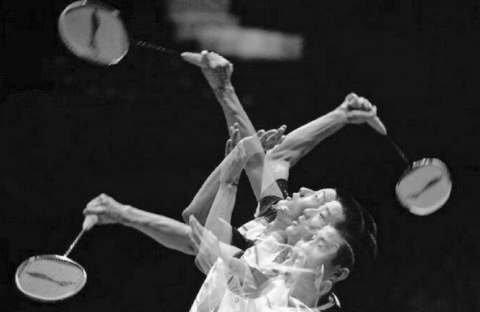
Figure 1. A sample image on stroking actions
Figure 2. The tracking errors of the three methods
This section verifies the effectiveness of the proposed feature extraction method through simulations on 30 badminton players in four scenarios. Before simulation, a dataset of badminton athlete action images was constructed. Every stroking process was captured by a fixed camera (shooting range: 5m), and the stroking arm was tagged. A total of 50 images and 399 videos were shot (Figure 1). Then, our method, template updating method, and least squares linear method were separately introduced to detect and track the stroking action trajectories in the collected images/videos on MATLAB. Figure 2 compares the tracking errors of the three methods.
As shown in Figure 2, the coordinates tracked by template updating method and least squares linear method deviated greatly from the real trajectory, while those tracked by our method only had a small error. The proposed method achieved better tracking effect than the contrastive methods. Table 1 compares the tracking success rates of the three methods.
It can be seen from Table 1 that the proposed method achieved a much higher tracking success rate than the two contrastive methods. The advantage of our method is attributed to the following factors: In our method, the contour of moving target is extracted, and a global matching approximation function is constructed as per the coordinates and size of the target; the trajectory of stroking actions is not predicted until the completion of these operations.
Table 1. The comparison of tracking success rates of the three methods
|
Method |
Total number of image pixels |
Total number of target pixels |
Total number of accurately tracked pixels |
Tracking success rate |
|
The proposed method |
500 |
317 |
305 |
0.96 |
|
Template updating method |
500 |
317 |
232 |
0.73 |
|
Least squares linear method |
500 |
317 |
251 |
0.79 |
The current trajectory tracking methods have difficulty in extracting the changing contour of the moving target, and generally face a high tracking error. To solve the problems, this paper proposes a feature extraction method for the action images of badminton players based on hierarchical features. Simulation results prove that the proposed method can accurately extract the salient features from the action images, and effectively track the moving target during the stroking process. The research results help to make badminton training more scientific and effective, and improve the techniques and tactics of badminton players.
[1] Haapasalo, H., Kannus, P., Sievänen, H., Pasanen, M., Uusi-Rasi, K., Heinonen, A., Oja, P., Vuori, I. (1998). Effect of long-term unilateral activity on bone mineral density of female junior tennis players. Journal of Bone and Mineral Research, 13(2): 310-319. https://doi.org/10.1359/jbmr.1998.13.2.310
[2] Balser, N., Lorey, B., Pilgramm, S., Naumann, T., Kindermann, S., Stark, R., Zentgraf, K., Williams, A.M., Munzert, J. (2014). The influence of expertise on brain activation of the action observation network during anticipation of tennis and volleyball serves. Frontiers in Human Neuroscience, 8: 568. https://doi.org/10.3389/fnhum.2014.00568
[3] Ivarsson, A., Stenling, A., Fallby, J., Johnson, U., Borg, E., Johansson, G. (2015). The predictive ability of the talent development environment on youth elite football players' well-being: A person-centered approach. Psychology of Sport and Exercise, 16: 15-23. https://doi.org/10.1016/j.psychsport.2014.09.006
[4] Khan, A.A., Shao, J., Ali, W., Tumrani, S. (2020). Content-aware summarization of broadcast sports videos: An audio–visual feature extraction approach. Neural Processing Letters, 52(3): 1945-1968. https://doi.org/10.1007/s11063-020-10200-3
[5] Wang, L., Sun, J., Li, T. (2020). Intelligent sports feature recognition system based on texture feature extraction and SVM parameter selection. Journal of Intelligent and Fuzzy Systems, 39(4): 4847-4858. https://doi.org/10.3233/JIFS-179970
[6] Ji, R. (2020). Research on basketball shooting action based on image feature extraction and machine learning. IEEE Access, 8: 138743-138751. https://doi.org/10.1109/10.1109/ACCESS.2020.3012456
[7] HimaBindu, G., Anuradha, C., Chandra Murty, P.S.R. (2019). Feature extraction techniques in associate with opposition based whale optimization algorithm. Ingénierie des Systèmes d’Information, 24(4): 403-410. https://doi.org/10.18280/isi.240407
[8] Li, T., Han, H. (2020). A high-performance basketball game forecast using magic feature extraction. Communications in Computer and Information Science, 1099 CCIS, 35-50. https://doi.org/10.1007/978-981-15-8760-3_3
[9] Yang, Z., Ren, H. (2019). Feature extraction and simulation of eeg signals during exercise-induced fatigue. IEEE Access, 7: 6389-46398. https://doi.org/10.1109/ACCESS.2019.2909035
[10] Satukumati S.B., Satla S., Kogila R. (2019). Feature extraction techniques for chronic kidney disease identification. Ingenierie des Systemesd'Information, 24(1): 95-99. https://doi.org/10.18280/isi.240114
[11] Jia, Y., Zhang, Q.F. (2015). Biomechanical analysis on the key motion technique of chinese elite female hammer throwers. China Sport Science and Technology, (2): 36-42.
[12] Handri, S., Nomura, S., Nakamura, K. (2011). Determination of age and gender based on features of human motion using AdaBoost algorithms. International Journal of Social Robotics, 3(3): 233-241. https://doi.org/10.1007/s12369-010-0089-0
[13] Zhong, J.Q., Wang, R.S. (2006). Multitemporal remote sensing images change detection based on linear feature. Journal-National University Of Defense Technology, 28(5): 80-83.
[14] Ying, W.J., Xu, K., Xu, S.P. (2017). Multi-objective trajectory planning of manipulator for badminton robot. Computer Engineering & Applications, 53(3): 258-265.
[15] Stoev, J., Gillijns, S., Bartic, A., Symens, W. (2010). Badminton playing robot-a multidisciplinary test case in mechatronics. IFAC Proceedings Volumes, 43(18): 725-731. https://doi.org/10.3182/20100913-3-US-2015.00028
[16] Depraetere, B., Liu, M., Pinte, G., Grondman, I., Babuška, R. (2014). Comparison of model-free and model-based methods for time optimal hit control of a badminton robot. Mechatronics, 24(8): 1021-1030. https://doi.org/10.1016/j.mechatronics.2014.08.001
[17] Wu, C.L., Han, C.Z. (2010). Tracking ballistic target based on square root quadrature Kalman filter. Control & Decision, 25(5):721-724, 729.
[18] Jiang, W.T., Liu, W.J., Yuan, H. (2013). Research of object tracking based on soft feature. Optik, 124(20): 4292-4295. https://doi.org/10.1016/j.ijleo.2013.01.042
[19] Zhang, L., Chen, W., Liu, J., Wen, C. (2015). A robust adaptive iterative learning control for trajectory tracking of permanent-magnet spherical actuator. IEEE Transactions on Industrial Electronics, 63(1): 291-301. https://doi.org/10.1109/TIE.2015.2464186