Indu Singh* | Rajni Jindal | Kanika Pandey | Kripali Agrawal | Kashish Kukreja
© 2020 IIETA. This article is published by IIETA and is licensed under the CC BY 4.0 license (http://creativecommons.org/licenses/by/4.0/).
OPEN ACCESS
Breast cancer causes a high percentage of mortality among women throughout the world. For improving breast cancer survival and results, early detection is important. The primary aim of the given study is to enhance the results of automated expert system (ES) in the field of medical diagnosis and come up with more accurate diagnosis system for breast cancer detection at early stage. This research introduces a new ensemble approach that accurately diagnose the breast cancer at a pre-developed stage. The recognized Wisconsin Diagnosis Breast Cancer (WDBC) dataset is used to provide raw breast cancer data in our study. Our proposed model rGWO-KSE (revised Grey Wolf Optimized SVM KNN Ensemble) implements an SVM-KNN ensemble and optimizes it with our newly introduced rGWO (revised Grey Wolf Optimization) technique. The performance of the proposed algorithm is evaluated based on several measures, e.g. accuracy, sensitivity, specificity, f-score and precision. Our model achieves 98.83 % accuracy in detection of breast cancer on WDBC dataset. The comparison with the previous studies for breast cancer detection proves that the proposed study provides better values for performance measures.
breast cancer diagnosis, ensemble learning, grey wolf optimization, K-nearest neighbor, support vector machine, weighted majority voting
Cancer refers to a massive group of diseases initiated by the growth and proliferation of abnormal cells that transcends the normal boundaries and spread to different organs affecting the adjoining body parts [1]. Prominently, cancer is named as eponym after the parts of body from where it originates; therefore, cancer that originates in the breast tissue is named as breast cancer.
Tumors are lumps of extra tissues which is a consequence of a bunch of rapidly dividing cells. Tumors are distinguished as cancerous or malignant and non-cancerous or benign. In benign tumor, cells do not spread to adjoining body parts. Proper medication and treatment are therefore not required for benign tumors. On the other side, in malignant tumors, cells divide uncontrolledly at a rapid rate occupying neighboring tissues and propagates to other sections of body resulting in adverse side effects. Therefore, breast cancer can also be referred as a malignant tumor that has developed and proliferated from cells in the breast [2].
According to the cancer statistics provided by the World Health Organization(WHO) (https://www.who.int/cancer/ prevention/diagnosis-screening/breast-cancer/en/), breast cancer affects 2.1 million women annually and is a major cause for deaths related to cancer amongst women. In 2018, it was estimated that breast cancer led to around 627,000 deaths amongst women, i.e., around 15% of deaths related to cancer amongst women. Although in developed regions, more women are affected by breast cancer, the breast cancer rates are also expanding rapidly in most of the regions globally.
According to the cancer statistics of United States [3], other than lung cancer, death rates due to breast cancer are more than any other cancer among women in United States (U.S.). Approximately 41,760 women are likely to die from breast cancer in the U.S in 2019. It is estimated that in the year 2019, approximately 30% of cancers diagnosed in women are breast cancers.
The drastic figures presented above can be depreciated by early diagnosis of cancer, i.e., classification of tumor into malignant and benign at pre-developed stage. Various expert systems and machine learning methods have proved to be of great help to doctors for diagnosis and classification of different types of cancers along with breast cancer. Different kinds of data mining algorithms, e.g. k Nearest Neighbors (KNN), Naive Bayes (NB), Support Vector Machine (SVM), Decision Tree (C4.5), [4] etc. have been applied to raw breast cancer data provided by Wisconsin Diagnosis Breast Cancer Data (explained in sec 3) for detecting and categorizing cancer into one of the categories-malignant or benign. The predictive model which is trustworthy and impeccable, providing high precision and accuracy, having the lowest fault and misclassification rates in terms of diagnosis and treatment is the primary objective for machine learning and data mining scholars and researchers.
The proposed model in the given study, i.e., revised Grey Wolf Optimized KNN SVM Ensemble (rGWO-KSE) attempts to analyze the data using six SVM and six KNN classifiers. The six SVM classifiers are differentiated on the basis of corresponding rbf values. The six KNN classifiers differs according to different k (nearest neighbors) values. The proposed revised Grey Wolf Optimization (rGWO) technique is the modified version of GWO which is used to provide weights to the twelve classifiers of weighted voting ensemble. It is prominent from the results presented in this study that the proposed algorithm could outperform the previous models for diagnosing breast cancer by accurately classifying tumor into appropriate categories. The proposed model provides 98.83% accuracy for WDBC dataset.
The remaining study is assembled in the following way. Few related works in similar domain has been discussed in Section 2. Section 3 provides the required knowledge regarding the machine learning algorithms that are applied in our model and WDBC dataset that provides the raw breast cancer data. The proposed model has been explained in Section 4. In Section 5, experimental results are being discussed on the basis of various performance metrics like accuracy, sensitivity, precision, f-score etc. which are obtained from the proposed model. Finally, Section 6 gives the future scope and conclusion for this study.
Like other medical diagnosis problems, classification systems are extensively employed in the domain of Breast Cancer (BC) diagnosis too. When the researches in the literature connected with this classification application are considered, it is evident that a huge variety of techniques were used which achieved high classification accuracies making use of the WDBC dataset taken from UCI repository.
Sarkar et al. [5] employed k-NN to classify Wisconsin-Madison breast cancer dataset. It produced 1.17% better classification result than the then best known results but suffered from large space and time complexities.
Bagui et al. [6] introduced a new generalization of multivariate k-RNN rule for BC diagnosis. With the help of two well-known datasets, they established that the computational complexity and performance of their proposed method was much better than the conventional k-nearest neighbor algorithm.
Wang et al. [7] proposed a new technique for neighborhood size selection of k-NN algorithm based on the idea of statistical confidence and tested their proposed approach on WDBC dataset. According to this method, number of nearest neighbors logically adjusts to reach a reasonable level of confidence. Additionally, the trade-off between the error rate and reject rate was stabilized by eliminating the patterns which had low confidence levels.
Sahan et al. [8] proposed a new hybrid model of fuzzy-artificial immune system (AIS) and k-nearest neighbor. They established the efficiency of their model against WDBC dataset via 10-fold cross-validation.
Li and Liu [9] introduced a kernel generating method where the new kernel focused on the correspondence of paired data in classes, where similarity of data is based on fuzzy theories. They were able to achieve better classification performance than Gaussian and polynomial kernels.
Chen et al. [10] proposed a rough set based SVM classifier for the diagnosis of breast cancer. They employed the rough set reduction algorithm for feature selection to extract the useful features and further improved the classification accuracy by SVM.
Stoean and Stoean [11] proposed a 2-step hybridized model for BC diagnosis and prognosis. First, learning and training part was performed by support vector machines and then a comprehensible impersonation of the resulting classification model was generated in propositional rules’ form.
Zheng et al. [12] classified the WDBC dataset using the extracted tumor features. They proposed a hybrid of K-Means and SVM to extract useful information and classify the tumor. K-means was used to identify the unknown patterns of the malignant and benign tumors resulting in a new feature which was based on the membership of the tumors to these patterns. SVM was then utilized to distinguish between the incoming tumors.
Onan [13] presented a hybrid classification model for automated diagnosis of breast cancer. It consisted of three phases: instance selection using weak gamma evaluator based fuzzy-rough instance selection, feature selection based on consistency method along with a re-ranking algorithm and classification using fuzzy-rough nearest neighbor. In the last phase, they used the fuzzy-rough nearest neighbor algorithm as this classifier does not need the optimal value of k.
Bashir et al. [14] proposed an ensemble framework of five classifiers: Naive Bayes, information gain based Decision tree, Memory based learner, Gini index based Decision tree and Support vector machine. The final prediction was determined using Weighted Majority voting where weights were assigned to a classifier based on its classification accuracy. The model was tested on four different datasets of breast cancer.
Wang et al. [15] proposed an ensemble learning algorithm based on SVM in order to increase the diagnosis accuracy while reducing the diagnosis variance of breast cancer. They proposed a hybrid of twelve different SVM classifiers based on Weighted Area Under the Receiver Operating Characteristic Curve Ensemble (WAUCE).
Abdar et al. [16] proposed a nested ensemble of Stacking and Voting to combine the classifiers in the ensemble for BC diagnosis. All nested ensemble classifiers consisted of metaclassifiers and classifiers. Metaclassifiers contained various classification techniques.
Cherif [17] optimized KNN algorithm by attribute filtering, clustering and refining using reliability coefficients for breast cancer diagnosis.
To classify unclustered breast cancer patients, Agrawal et al. [18] introduced an ensemble classification step succeeding the ensemble clustering step. They put to use a step by step pipeline that combined ensemble classification with ensemble clustering to recognize the core groups and their data distribution.
3.1 K-nearest neighbors
One of the most simple and effective multi-class classification technique, K-nearest neighbors is an instance-based learning method. KNN is a non-parametric technique which does not require a learning phase. The classifier model is developed by associating a distance function with the training sample and the choice function of a class which is based on the k classes.
Using a similarity measure such as Euclidean distance, every new element is classified by comparing it with k of its nearest neighbors or elements. The element then identifies with the class to which most of its neighbors belong.
Consider k pairs of samples and target (α1, β1), (α2, β2), …, (αk, βk) where $\alpha_{\mathrm{i}} \epsilon \mathrm{R}^{\mathrm{d}}$and $\beta_{\mathrm{i}} \epsilon\{0,1\}$, then according to Euclidean distance the distance between the two data points can be computed as:
$\mathrm{d}^{2}\left(\alpha_{\mathrm{i}}, \alpha_{\mathrm{j}}\right)=\left\|\alpha_{\mathrm{i}}-\alpha_{\mathrm{j}}\right\|^{2}=\sum_{z=1}^{d}\left(\alpha_{i z}-\alpha_{j z}\right)^{2}$ (1)
The parameter k determines the number of neighbors whose distances are compared with the object to be classified. The accuracy of the classifier depends on the value of this parameter.
3.2 Support vector machine
With high generalization ability, SVM is one of the most effective binary classification techniques. Introduced by Vapnik et al. [19] in the 1990s, SVM aims towards minimizing structural risk which makes the model strongly resistant to overfitting. A model can be considered an overfit if it classifies testing or unseen data with a substantially lower accuracy than the training data.
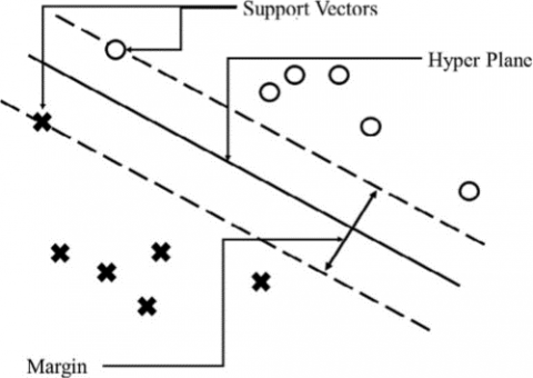
SVM classifies the data into different classes by constructing a hyperplane or a set of hyperplanes. In SVM a hyper-plane is described as a surface that completely partitions the data points in two classes such that no data point of a class falls into the other side of the hyperplane, as shown in Figure 1. Out of an infinite number of possible hyperplanes, the one with the maximum distance to the closest data points of both classes is considered the most optimal [19].
A hyperplane is the set of points $\vec{x}$ satisfying the equation:
$\vec{w} \cdot \vec{x}+b=0$ (2)
where, b is the bias and w is the weight vector which in linear case can be easily solved using Lagrangian multipliers.
Though initially introduced for linearly separable cases, SVM can effectively classify high dimensional data by mapping it onto a high dimensional feature space such that the mapped data can be easily separated using lower-order polynomial functions. The mapping of original data to a high dimensional feature space is performed by a kernel function [20].where, b is the bias and w is the weight vector which in linear case can be easily solved using Lagrangian multipliers.
Figure 1. Linear SVM classifier [21]
The following common kernels are used in SVM classifier:
1. Linear Kernel:
$f\left(\alpha_{i}, \alpha_{j}\right)=\alpha_{i} \alpha_{j}$ (3)
2. Polynomial Kernel:
$\mathrm{f}\left(\alpha_{\mathrm{i}}, \alpha_{\mathrm{j}}\right)=\left(\beta \alpha^{\mathrm{t}} \alpha_{\mathrm{j}}+\mathrm{r}^{2}\right)^{2}$ (4)
3. RBF Kernel:
$\mathrm{f}\left(\alpha_{\mathrm{i}}, \alpha_{\mathrm{j}}\right)=\exp \left[\gamma\left\|\alpha_{\mathrm{i}}-\alpha_{\mathrm{j}}\right\|^{2}\right]$ (5)
4. Sigmoid Kernel:
$\mathrm{f}\left(\alpha_{\mathrm{i}}, \alpha_{\mathrm{j}}\right)=\tanh \left(\beta \alpha_{\mathrm{i}}^{\mathrm{t}} \alpha_{\mathrm{j}}+\mathrm{r}\right)$ (6)
3.3 Ensemble learning
One of the most remarkable approaches for improving the overall performance of individual classifiers is combining them through various techniques. This is known as ensemble learning. An ensemble consists of a number of classifiers with individual decisions that are combined by various mechanisms such as voting or other techniques to group and classify instances resulting in more accurate decisions than those of individual classifiers [22].
The votes from different classifiers can be combined in a number of ways, the most common being the majority vote ensemble in which each classifier gives a binary vote of 0 or 1. A more sophisticated approach is to give different weightage to each classifier’s vote which leads to a reduction in number of mistakes made by the ensemble [23]. This is known as weighted majority ensemble, in which each classifier’s vote is given an optimal weightage in order to get better results.
Two very common techniques in this learning are Bagging and Boosting, which use many weaker predictors to obtain better results. In bagging, the training data set is replicated n times using bootstrapping; and n independent classifiers are constructed by resampling the original training datasets randomly, with replacements. In Boosting too, the ensemble is made by resampling the training data with n individual classifiers which can then be combined by different techniques. But in this technique, unlike bagging, the n classifiers, are sequentially trained.
3.4 Grey wolf optimization
Proposed by Mirjalili et al. [24], GWO is an efficient population based meta heuristic optimization technique. Inspired by the leadership hierarchy and preying techniques of grey wolves, wolves are ranked according to their mental talents into four major categories viz. alpha, beta, delta, omega (Figure 2).
Figure 2. Grey Wolf Hierarchy (dominance decreases downwards) [24]
The process of hunting includes searching, encircling and attacking the prey [24]. Encircling of prey according to conventional GWO is simulated as follows:
$\vec{D}=\left|\vec{C} \cdot \vec{X}_{\mathrm{p}}(\mathrm{t})-\vec{X}(\mathrm{t})\right|$ (7)
$\vec{X}(\mathrm{t}+1)=\vec{X}_{\mathrm{p}}(\mathrm{t})-\vec{A} \cdot \vec{D}$ (8)
t marks the current iteration, $\vec{A}$ and $\vec{C}$ are random chosen coefficients vectors, $\overrightarrow{X_{p}}$ tells the prey’s location. $\vec{X}$ contains wolves’ positions. The coefficient vectors $\vec{A}$ and $\vec{C}$ are calculated as:
$\vec{A}=2 \vec{a} \cdot \vec{r}_{1}-\vec{a}$ (9)
$\vec{C}=2 \vec{r}_{2}$ (10)
where elements of vectors $\vec{a}$ are linearly decreased from 2 to 0 with the update Eq. (11) and $\overrightarrow{r 1}$ and $\overrightarrow{r 2}$ are random vectors have values in range of [0, 1].
$\vec{a}=2(1-\mathrm{t} / \mathrm{T})$ (11)
where, t marks the current iteration and T is the maximum iterations.
In the process of hunting, the better wolves are initially assumed to have better knowledge regarding the location of the prey and thus lead the pack. So, the top three candidate solutions in every iteration are made the alpha, beta and delta wolves respectively [24]. Other wolves update their positions with respect to the best ones. Positions of wolves are updated as per the following formulae:
$\vec{D}_{\alpha}=\left|\vec{C}_{1} \cdot \vec{X}_{\alpha}-\vec{X}\right|$ (12)
$\vec{D}_{\beta}=\left|\vec{C}_{1} \cdot \vec{X}_{\beta}-\vec{X}\right|$ (13)
$\vec{D}_{\delta}=\left|\vec{C}_{1} \cdot \vec{X}_{\delta}-\vec{X}\right|$ (14)
$\vec{X}_{1}=\vec{X}_{\alpha}-\vec{A}_{1} \cdot \vec{D}_{\alpha}$ (15)
$\vec{X}_{2}=\vec{X}_{B}-\vec{A}_{2} \cdot \vec{D}_{\beta}$ (16)
$\vec{X}_{3}=\vec{X}_{\delta}-\vec{A}_{3} \cdot \vec{D}_{\delta}$ (17)
$\vec{X}(\mathrm{t}+1)=\left(\vec{X}_{1}+\vec{X}_{2}+\vec{X}_{3}\right) / 3$ (18)
3.5 Wisconsin diagnosis breast cancer (WDBC) dataset
The efficacy of our proposed model is tested upon the standard Wisconsin Diagnosis Breast Cancer dataset [25] from University of California. This dataset includes 699 instances divided into two classes: benign (negative class) and malignant (positive class). The dataset has ten features that are used to describe the instances. Sixteen records with missing values are removed during data preprocessing. The feature distribution of the dataset is summarized in Table 1.
Table 1. Description of the WDBC dataset [25]
|
Feature No |
Feature Description |
Values of attributes |
Mean |
Standard error of mean |
Standard Deviation |
Variance |
|
1 |
Clump thickness |
1-10 |
4.418 |
0.107 |
2.816 |
7.928 |
|
2 |
Uniformity of cell size |
1-10 |
3.134 |
0.115 |
3.051 |
9.311 |
|
3 |
Uniformity of cell shape |
1-10 |
3.207 |
0.112 |
2.972 |
8.832 |
|
4 |
Marginal adhesion |
1-10 |
2.807 |
0.108 |
2.855 |
8.153 |
|
5 |
Single epithelial cell size |
1-10 |
3.216 |
0.084 |
2.214 |
4.903 |
|
6 |
Bare nuclei |
1-10 |
3.464 |
0.138 |
3.641 |
13.255 |
|
7 |
Bland chromatin |
1-10 |
3.438 |
0.092 |
2.438 |
5.946 |
|
8 |
Normal nucleoli |
1-10 |
2.867 |
0.115 |
3.054 |
9.325 |
|
9 |
Mitoses |
1-10 |
1.589 |
0.065 |
1.715 |
2.941 |
4.1 Working of our proposed model
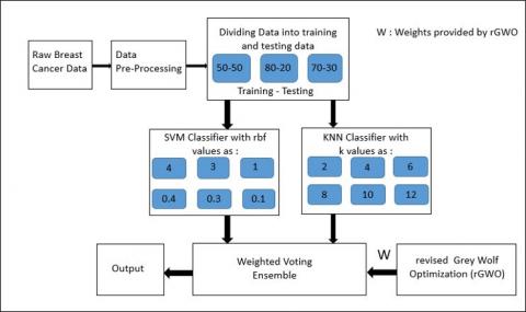
The architecture of the proposed rGWO-KSE (revised Grey Wolf Optimized SVM KNN Ensemble) model is given in Figure 3. Algorithm 2 illustrates the pseudocode for rGWO-KSE.
In the first step, raw breast cancer data is taken from Wisconsin Diagnosis Breast Cancer dataset and the data is pre-processed by removing the missing values. Therefore, 16 records are removed having missing values and the remaining study is conducted using 683 records. Initially, 50% data is considered for training whereas 50% data is used to test the proposed model.
In the second step, data is trained using SVM expert system. The best outcomes are produced by SVM when we use RBF kernel function for classification [26]. It has been proved from the experimental results that using the RBF kernel function, the performance of SVM expert system will diverge with the choice of RBF function. Therefore, to ensure the maximum utilization of SVM classifier, we are training six different kinds of SVM experts with varied values of RBF parameters. This methodology guarantees high variation of classifiers in the ensemble classification.
Values designated to the rbf variable for different SVM classifiers are [1, 3, 4, 0.1, 0.3, 0.4].
Later, in the result section, it has been demonstrated that the performance measures of each SVM classifier differs, based on the selected RBF value.
In the third step, the data is trained using KNN expert system. To ensure the compatibility with the SVM classifier, the structure of KNN classifier is similar to the SVM classifier. Compatibility and synchronization between these two expert systems enable us to collaborate them to perform ensemble classification. The parameter k in the KNN expert depicts the no. of neighbors closest or nearest to the certain observation in validation dataset. Variation in k parameter impacts performance measures of all KNN experts.
In order to guarantee maximum utilization of KNN classifier and to provide greater diversity, we are training six KNN classifiers having distinct k parameter values. Six KNN experts have different k parameters with values: [2, 4, 6, 8, 10, 12].
In the fourth step, the outcomes of SVM and KNN expert systems are ensembled using weighted majority voting (WMV). Littlestone and Warmuth [23] demonstrated the minimization of errors made by the ensemble system by providing weights to the majority voting procedure as the majority voting process is instinctive.
Figure 3. Architecture of the proposed model rGWO-KSE
In this study, we use weighted voting technique to combine the outcomes of the SVM and KNN experts in the ensemble. All the experts are provided weights based on their classification accuracy.
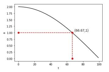
We have proposed the revised Grey Wolf Optimization (rGWO) algorithm to generate weights for the twelve (SVM and KNN) experts for WMV. In the conventional GWO [25], 50% iterations are used to explore the prey whereas another 50% iterations are used for exploiting the prey, overseeing the correct balance amidst exploring and exploiting for accurately estimating the globally optimal solution as shown in Figure 4.
Figure 4. Variation of a in original GWO
Figure 5. Variation of a in rGWO
The vector $\vec{a}$ in original GWO [24] is calculated using (11) $\vec{a}$= 2(1 − t/T).
Figure 4 demonstrates that element a decreases linearly from 2 to 0. Thus, an exponential function can be used to overcome this shortcoming.
In order to maintain a proper balance of iterations for exploration and exploitation, our proposed rGWO (revised Grey Wolf Optimization) algorithm uses trigonometric (cosine) function which is a continuous and exponential function, for calculating $\vec{a}$. We have revised the equation of $\vec{a}$ as:
$\vec{a}=2 \cos (t \pi / 2 T)$ (19)
The vector $\vec{a}$ decreases exponetially from 2 to 0 as shown in Figure 5 with approximately 67% of iterations dedicated to exploration and around 33% iterations dedicated to exploitation resulting in an accurate estimation of global optimum.
Since sine function is also a continuous and exponential function, it can also be used for calculating $\vec{a}$ as:
$\vec{a}=2(1-\sin (t \pi / 2 T))$ (20)
Figure 6. Variation of a in sin-GWO
We used cosine function to calculate $\vec{a}$ against sine function offers less exploration (approx 33%) than exploitation (approx 67%) (Figure 6), which is even worse than the original GWO and therefore fails to provide a better global optimum.
The pseudocode for rGWO is shown in Algo 1.
|
Algorithm 1: Helper rGWO function for Algorithm 2 |
|
initialize the following: Xi(i=1,2, ..., n), a, A, C, iterations, Xα, Xβ, Xγ, t; while t ≤ iterations do foreach i $\in$[0, n] do Compute fitness of agent i end Xα = best solution Xβ = second best solution Xγ = third best solution a = 2cos($t \pi$ /2T ) t = t + 1 foreach i $\in$[0, n] do $\mathrm{A}=2 \vec{a} \cdot \vec{r}_{1}-\vec{a}$ where $\vec{r}_{1} \in[0,1]$ $\mathrm{C}=2 \vec{r}_{2}$ where $\vec{r}_{2} \in[0,1]$ update agent’s position end end |
Using rGWO, the set of weight coefficients is described, where each component j depicts weight for jthclassifier in an ensemble, i.e., w = (w1, w2, ..., w12) based on the accuracy of individual experts in classifying the training data.
The outcomes obtained from the twelve classifiers are multiplied with the corresponding weights given by rGWO and the final result is their summation as shown in Eq. (21).
$\mathrm{y}=\sum_{i=1}^{j=12} w_{j \cdot} j_{\mathrm{y}}$ (21)
|
Algorithm 2: Algorithm for rGWO-KSE |
|
initialize the following: rbfi= {1, 3, 4, 0.1, 0.3, 0.4}, ki = {2, 4, 6, 8, 10, 12} foreach i $\epsilon$[0, n] do $S V M_{i}=\exp \left[\gamma\left\|X_{i}-X_{j}\right\|^{2}\right]$ $K N N_{i}=\sum_{z=1}^{d}\left(X_{i}-X_{j}\right)^{2}$ end wts = rGWO( KNN1, ……, KNN6, SVM1……SVM6) where wts = (w1, ………., w12) final predicton = majority (w1(KNN)), ….., w6(KNN6), w1(SVM1,. … w12 (SVM6)) end |
The prediction that we get from the weighted majority of the models is taken as the final prediction or the final output.
Similarly, we execute the above experiment for 80% training and 20% testing data and 70% training and 30% testing data.
This section concentrates on evaluating the performance measures of base classifiers, i.e., SVM and KNN as well as the revised Grey Wolf Optimized Ensemble in terms of accuracy, specificity, sensitivity, precision and f-measure. The opinion of each classifier in the ensemble is taken into consideration by means of Weighted Majority Voting (WMV). The weight given to each classifier is proportional to its individual accuracy. Finally, a comparison is made between the proposed model and the previous studies related to the similar domain.
5.1 Measures for performance evaluation
We have evaluated the performance of the classifiers using the following metrics for data classification:
where, TN, TP, FP and FN represent the number of true negatives, true positives, false positives and false negatives, respectively.
5.2 Evaluating the performance of individual classifiers of KNN and SVM in terms of accuracy
The performance of individual classifiers of KNN for different values of k as well as of SVM for different values of rbf is compared in terms of accuracy. The fitness function provided to the rGWO algorithm depends on accuracy of the classifiers.
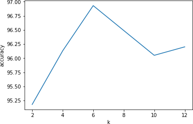
In KNN algorithm, increasing the value of k increases the training error (increase bias), however the test error (decrease variance) is reduced at the same time. For k=1, the resolution becomes too fine that it tends to overfit the data and results in least accuracy whereas the highest accuracy of 96.93% is obtained when k is neither too low nor too high, i.e., k=5 as shown in Figure 7.
Figure 7. Accuracy of KNN experts for different values of k
Figure 8. Accuracy of SVM experts for different values of rbf kernel
The accuracy of SVM experts vary inversely with the value of rbf parameter as shown in Figure 8. Therefore, the weights provided to the classifiers decrease with increase in rbf parameter.
5.3 Majority voting ensemble vs weighted voting ensemble using rGWO
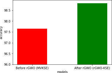
A comparison between accuracies of majority voted KNN SVM ensemble (MVKSE) and weighted voting using revised grey wolf optimization (rGWO-KSE) is shown in Figure 9. We observed a significant increase in accuracy from 97.65% to 98.83% after introducing weights in the ensemble technique.
Figure 9. Comparison of accuracy of MVKSE and rGWO-KSE
5.4 Evaluating the performance of GWO for different values of $\vec{a}$
Table 2. Variation of accuracy with different formulas for $\vec{a}$
|
Type of GWO |
Formula for $\vec{a}$ |
Accuracy (%) |
|
Original GWO |
2(1- t/T) |
98.24 |
|
Original GWO |
2(1-sin(t π/2T)) |
97.36 |
|
rGWO |
2cos(t π/2T) |
98.83 |
5.5 Overall comparison
The overall comparison of individual classifiers of KNN as well as of SVM and their optimized ensemble in terms of accuracy, sensitivity, specificity, precision and f-measure is depicted in Table 3.
According to our proposed model, the base classifier KNN with k=1 results in the minimum sensitivity or least number of true positives as proved by 91.24 sensitivity as per Figure 10 whereas the highest sensitivity, i.e., 100 is obtained when we implemented SVM classifiers with rbf=5, rbf=2, rbf=1 and rbf=0.5 individually, i.e., these base classifiers classify all the positives in their corresponding class but they fail to produce the highest specificity and therefore fail to have the highest accuracy.
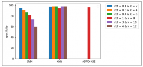
Similarly as per Figure 11, the highest specificity with KNN classifier is obtained when k=9 and k=5 and with SVM classifier, it is achieved when rbf parameter is 0.1, i.e., these classifiers classify maximum true negatives to their corresponding class but they fail to have the highest sensitivity or do not classify positives to their true class accurately and therefore fail to have the highest accuracy.
Since our proposed rGWO-KSE model balances the specificity and sensitivity, it results in the highest accuracy in comparison to the individual experts as illustrated in Table 3.
Precision measures, what percentage of patients predicted as cancerous, are actually having cancer. The people diagnosed with breast cancer are summation of FP and TP and people that have breast cancer in actual are TP. It can be observed that our proposed rGWO-KSE algorithm improves the precision of base classifiers by incorporating them into an ensemble as shown in Figure 12.
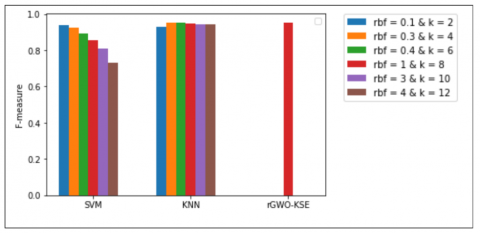
F-measure increases with lesser false positives and lesser false negatives and ensures that false alarms do not disturb the model. Figure 13 clearly depicts that the ensemble of SVM and KNN classifiers improves the f-measure of the individual classifiers.
Table 3. Comparison of accuracy, sensitivity, specificity, precision & F-measure between different classifiers
|
Classifiers |
rbf / k |
Accuracy |
Sensitivity |
Specificity |
Precision |
F-measure |
|
SVM |
4 |
74.06 |
100 |
60.07 |
57.83 |
73.17 |
|
SVM |
3 |
82.87 |
100 |
73.63 |
68.20 |
80.78 |
|
SVM |
1 |
87.99 |
100 |
81.53 |
75.48 |
85.74 |
|
SVM |
0.4 |
91.51 |
100 |
86.94 |
81.04 |
89.37 |
|
SVM |
0.3 |
94.15 |
99.58 |
91.22 |
86.44 |
92.42 |
|
SVM |
0.1 |
95.47 |
98.32 |
94.92 |
90.01 |
93.94 |
|
KNN |
2 |
95.18 |
91.24 |
97.30 |
94.92 |
92.88 |
|
KNN |
4 |
96.63 |
94.98 |
97.53 |
95.57 |
95.16 |
|
KNN |
6 |
96.93 |
95.40 |
97.75 |
93.68 |
95.15 |
|
KNN |
8 |
96.49 |
94.57 |
97.53 |
95.58 |
94.43 |
|
KNN |
10 |
96.05 |
92.90 |
97.75 |
95.89 |
94.15 |
|
KNN |
12 |
96.20 |
93.74 |
97.53 |
95.53 |
94.43 |
|
rGWO-KSE |
– |
98.83 |
97.07 |
96.40 |
96.01 |
95.31 |
Figure 10. Sensitivity of different classifiers along with our rGWO-KSE model
Figure 11. Specificity of different classifiers along with our rGWO-KSE model
Figure 12. Precision of different classifiers along with our rGWO-KSE model
Figure 13. F-measure of different classifiers along with our rGWO-KSE model
5.6 Dataset distribution
The distribution of data between training and testing plays a significant role in determining the effectiveness of the model.
As shown in Table 4, our model rGWO-KSE provides 98.83% accuracy for 50-50% training-test partition, 99.02% accuracy for 70-30% training-test partition and 99.27% accuracy for 80-20% training-test partition based on the WDBC dataset.
Table 4. Variation of accuracy with dataset
|
Dataset Distribution |
Accuracy (%) |
|
50-50 |
98.83 |
|
70-30 |
99.02 |
|
80-20 |
99.27 |
To demonstrate the effectiveness of our proposed model, the results acquired from our proposed approach are compared with the results from some recently developed models (from 2010 to 2020) in terms of accuracy. Some related studies in the similar domain are discussed which have applied their algorithms on the WDBC dataset as shown in Table 5. Some of the models have been able to attain significant accuracies. Sheikhpour et al. [28] proposed a model by applying Particle Swarm Optimization with non-parametric Kernel Density Estimation and attained a notable accuracy of 98.45%. Abdar et al. [16] achieved a comparable accuracy of 98.07% by implementing a nested ensemble approach that utilized the Stacking and Voting techniques among the classifiers. Our proposed model obtains the highest accuracy of 98.83% for the breast cancer diagnosis.
Table 5. Comparison of our proposed model with previous studies
|
S. No. |
Study |
Year |
Algorithm |
Accuracy (%) |
|
1 |
D.C Li et al. [9] |
2010 |
SVM CPBK |
93.26 |
|
2 |
Stoean & Stoean [11] |
2013 |
SVM and revolutionary |
97.23 |
|
3 |
Saez et al. [27] |
2014 |
ML with KNN |
96.14 |
|
4 |
Zheng et al. [12] |
2014 |
K-means & SVM |
97.38 |
|
5 |
Bashir et al. [14] |
2015 |
Weighted Vote based ensemble |
95.09 |
|
6 |
Sheikhpour et al. [28] |
2016 |
PSO-KDE |
98.45 |
|
7 |
Nilashi et al. [29] |
2017 |
Knowledge Based System using Fuzzy Logic |
93.2 |
|
8 |
Abdar et al. [16] |
2018 |
Nested ensemble approach |
98.07 |
|
9 |
Wuniri et al. [30] |
2019 |
BIG-F |
97.1 |
|
10 |
Sadhukhan et al. [31] |
2020 |
SVM+KNN+Image Processing |
97.49 |
|
11 |
Our Proposed Model |
2020 |
rGWO-KSE |
98.83 |
In the given study, we have proposed rGWO-KSE (revised Grey Wolf Optimized KNN SVM Ensemble) model for the diagnosis of breast cancer by differentiating tumor as malignant or benign at a pre-mature stage. For this, we utilized the renowned WDBC dataset [25] from UCI dataset repository to obtain raw breast cancer data. The proposed rGWO-KSE model includes six SVM (differentiated by RBF parameter) and six KNN classifiers (differentiated by k parameter) and incorporates them into a weighted voting ensemble. The proposed rGWO (revised Grey Wolf Optimization) technique is used to provide weights to the twelve classifiers. The rGWO technique differs from the original GWO in terms of update equation of $\vec{a}$. The proposed rGWO-KSE model achieves an accuracy of 98.83% on WDBC dataset of UCI repository.
In future, the proposed rGWO-KSE model can be applied to different domains in medical research.
[1] Hejmadi, M. (2014). Introduction to Cancer Biology, Bookboon.
[2] Khuwaja, G.A., Abu-Rezq, A. (2004). Bimodal breast cancer classification system. Pattern Analysis and Applications, 7(3): 235-242. https://doi.org/10.1007/BF02683990
[3] DeSantis, C.E., Ma, J., Gaudet, M.M., Newman, L.A., Miller, K.D., Goding Sauer, A., Jemal, A., Siegel, R.L. (2019). Breast cancer statistics. CA: A Cancer Journal for Clinicians, 69(6): 438-451.
[4] Asri, H., Mousannif, H., Al Moatassime, H., Noel, T. (2016). Using machine learning algorithms for breast cancer risk prediction and diagnosis. Procedia Computer Science, 83: 1064-1069.
[5] Sarkar, M., Leong, T.Y. (2000). Application of k-nearest neighbors algorithm on breast cancer diagnosis problem. Proc. AMIA Symp., pp. 759-763.
[6] Bagui, S.C., Bagui, S., Pal, K., Pal, N.R. (2003). Breast cancer detection using rank nearest neighbor classification rules. Pattern Recognition, 36(1): 25-34. https://doi.org/10.1016/S0031-3203(02)00044-4
[7] Wang, J., Neskovic, P., Cooper, L.N. (2006). Neighborhood size selection in the k-nearest-neighbor rule using statistical confidence. Pattern Recognition, 39(3): 417-423. https://doi.org/10.1016/j.patcog.2005.08.009
[8] Şahan, S., Polat, K., Kodaz, H., Güneş, S. (2007). A new hybrid method based on fuzzy-artificial immune system and k-nn algorithm for breast cancer diagnosis. Computers in Biology and Medicine, 37(3): 415-423. https://doi.org/10.1016/j.compbiomed.2006.05.003
[9] Li, D.C., Liu, C.W. (2010). A class possibility based kernel to increase classification accuracy for small data sets using support vector machines. Expert Systems with Applications, 37(4): 3104-3110. https://doi.org/10.1016/j.eswa.2009.09.019
[10] Chen, H.L., Yang, B., Liu, J., Liu, D.Y. (2011). A support vector machine classifier with rough set-based feature selection for breast cancer diagnosis. Expert Systems with Applications, 38(7): 9014-9022. https://doi.org/10.1016/j.eswa.2011.01.120
[11] Stoean, R., Stoean, C. (2013). Modeling medical decision making by support vector machines, explaining by rules of evolutionary algorithms with feature selection. Expert Systems with Applications, 40(7): 2677-2686. https://doi.org/10.1016/j.eswa.2012.11.007
[12] Zheng, B., Yoon, S.W., Lam, S.S. (2014). Breast cancer diagnosis based on feature extraction using a hybrid of k-means and support vector machine algorithms. Expert Systems with Applications, 41(4): 1476-1482. https://doi.org/10.1016/j.eswa.2013.08.044
[13] Onan, A. (2015). A fuzzy-rough nearest neighbor classifier combined with consistency-based subset evaluation and instance selection for automated diagnosis of breast cancer. Expert Systems with Applications, 42(20): 6844-6852. https://doi.org/10.1016/j.eswa.2015.05.006
[14] Bashir, S., Qamar, U., Khan, F.H. (2015). Heterogeneous classifiers fusion for dynamic breast cancer diagnosis using weighted vote-based ensemble. Quality & Quantity, 49(5): 2061-2076. https://doi.org/10.1007/s11135-014-0090-z
[15] Wang, H., Zheng, B., Yoon, S.W., Ko, H.S. (2018). A support vector machine-based ensemble algorithm for breast cancer diagnosis. European Journal of Operational Research, 267(2): 687-699. https://doi.org/10.1016/j.ejor.2017.12.001
[16] Abdar, M., Zomorodi-Moghadam, M., Zhou, X., Gururajan, R., Tao, X., Barua, P. D., Gururajan, R. (2018). A new nested ensemble technique for automated diagnosis of breast cancer. Pattern Recognition Letters, 132: 123-131. https://doi.org/10.1016/j.patrec.2018.11.004
[17] Cherif, W. (2018). Optimization of k-nn algorithm by clustering and reliability coefficients: Application to breast-cancer diagnosis. Procedia Computer Science, 127: 293-299. https://doi.org/10.1016/j.procs.2018.01.125
[18] Agrawal, U., Soria, D., Wagner, C., Garibaldi, J., Ellis, I.O., Bartlett, J.M., Cameron, D., Rakha, E.A., Green, A.R. (2019). Combining clustering and classification ensembles: A novel pipeline to identify breast cancer profiles. Artificial Intelligence in Medicine, 97: 27-37. https://doi.org/10.1016/j.artmed.2019.05.002
[19] Cortes, C., Vapnik, V. (1995). Support-vector networks. Machine Learning, 20(3): 273-297. https://doi.org/10.1007/BF00994018
[20] Boser, B.E., Guyon, I.M., Vapnik, V.N. (1992). A training algorithm for optimal margin classifiers. In: Proceedings of the Fifth Annual Workshop on Computational Learning Theory, pp. 144-152. https://doi.org/10.1145/130385.130401
[21] Tao, D., Tang, X., Li, X., Wu, X. (2006). Asymmetric bagging and random sub-space for support vector machines-based relevance feedback in image retrieval. IEEE Transactions on Pattern Analysis and Machine Intelligence, 28(7): 1088-1099. https://doi.org/10.1109/TPAMI.2006.134
[22] Dietterich, T.G. (1997). Machine-learning research. AI Magazine, 18(4): 97-97. https://doi.org/10.1609/aimag.v18i4.1324
[23] Littlestone, N., Warmuth, M.K. (1994). The weighted majority algorithm. Information and Computation, 108(2): 212-261. https://doi.org/10.1006/inco.1994.1009
[24] Mirjalili, S., Mirjalili, S.M., Lewis, A. (2014). Grey wolf optimizer. Advances in Engineering Software, 69: 46-61. https://doi.org/10.1016/j.advengsoft.2013.12.007
[25] Wolberg, W.H., Street, W.N., Mangasarian, O.L. (1992). Breast cancer wisconsin (diagnostic) data set. UCI Machine Learning Repository. http://archive.ics.uci.edu/ml/.
[26] Kuang, F., Xu, W., Zhang, S. (2014). A novel hybrid KPCA and SVM with Ga model for intrusion detection. Applied Soft Computing, 18: 178-184. https://doi.org/10.1016/j.asoc.2014.01.028
[27] Sáez, J.A., Derrac, J., Luengo, J., Herrera, F. (2014). Statistical computation of feature weighting schemes through data estimation for nearest neighbor classifiers. Pattern Recognition, 47(12): 3941-3948. https://doi.org/10.1016/j.patcog.2014.06.012
[28] Sheikhpour, R., Sarram, M.A., Sheikhpour, R. (2016). Particle swarm optimization for bandwidth determination and feature selection of kernel density estimation based classifiers in diagnosis of breast cancer. Applied Soft Computing, 40: 113-131. https://doi.org/10.1016/j.asoc.2015.10.005
[29] Nilashi, M., Ibrahim, O., Ahmadi, H., Shahmoradi, L. (2017). A knowledge-based system for breast cancer classification using fuzzy logic method. Telematics and Informatics, 34(4): 133-144. https://doi.org/10.1016/j.tele.2017.01.007
[30] Wuniri, Q., Huangfu, W., Liu, Y., Lin, X., Liu, L., Yu, Z. (2019). A generic-driven wrapper embedded with feature-type-aware hybrid bayesian classifier for breast cancer classification. IEEE Access, 7: 119931-119942. https://doi.org/10.1109/ACCESS.2019.2932505
[31] Sadhukhan, S., Upadhyay, N., Chakraborty, P. (2020). Breast Cancer Diagnosis Using Image Processing and Machine Learning. In: Mandal J., Bhattacharya D. (eds) Emerging Technology in Modelling and Graphics. Advances in Intelligent Systems and Computing, vol 937. Springer, Singapore, 113-127. https://doi.org/10.1007/978-981-13-7403-6_12