Wei Liu
OPEN ACCESS
In the era of the big data, the accurate prediction of real-time traffic flow is essential to making rational decisions on travel time, cost and route. To forecast traffic flow accurately, this paper firstly analyzes the features of traffic data, and proves that the traffic data collected from an overpass are self-similar. For simplicity, the long-term correlation (LTC) time series of the traffic data were decomposed into short-term correlation (STC) product functions (PFs) through local mean decomposition (LMD). On this basis, a traffic flow prediction model was developed based on the generalized autoregressive conditional heteroskedasticity (GARCH) model. Simulation results show that our model was more accurate in predicting traffic flow than the original GARCH and the autoregressive integrated moving average (ARIMA) model. Therefore, this research provides a suitable tool for the prediction of traffic flow.
time series, traffic data, big data technology, local mean decomposition (LMD), generalized autoregressive conditional heteroskedasticity (GARCH) model
Traffic big data contains a huge amount of information, which needs to be mined effectively according to the demand. The effective processing of traffic big data can effectively improve traffic operation efficiency, reduce traffic congestion time, promote intelligent traffic management, and reduce time cost and capital cost.
The prediction of traffic flow is essential to making rational decisions on travel time, cost and route. There are many models to predict the traffic flow. Each of them has its strengths and defects. The most popular traffic flow prediction models are based on statistical theories, including time series model [1] and Kalman filter model [2-3].
The time series model was first adopted by Ahmed et al. to predict traffic flow in 1982 [4]. The model was improved by Ghosh et al. to forecast seasonable traffic flow [5]. The improved time series model can project changing traffic flow more accurately than the original model. For Kalman filter model, Yang et al. [6] designed a multi-step traffic flow prediction method based on this model, and proved that the method has high prediction accuracy. Muruganantham et al. [7] improved the Kalman filter model to optimize the parameters of dynamic traffic flow prediction model in an accurate and robust manner.
The traffic flow prediction models are often coupled with nonlinear theories [8-10], such as wavelet analysis, fractal theory, chaos theory and catastrophe theory. For example, Kumar et al. [11] processed traffic data through local mean decomposition (LMD), and then predicted the traffic flow by the autoregressive integrated moving average (ARIMA) model. Jin et al. [12] combined the Kalman filter and Gaussian process-based hybrid model into a traffic flow prediction model, which inherits the real-time performance of the Kalman filter and the high accuracy of the hybrid model.
The prediction of traffic flow can also be improved by state-of-the-art technologies like the support vector machine (SVM) [13] and neural networks (NNs). Among them, the SVM can predict trends and generalize solutions accurately, offering a desirable tool to process high-dimensional small samples. Based on the SVM, Huan et al. [14] designed an improved prediction model, which can forecast traffic flow accurately online. Yao et al. [15] proposed a dynamic traffic flow prediction model based on an NN. Guo et al. [16] improved the prediction accuracy of the traditional NN model, using the origin-destination (OD) matrix.
The rapid development of big data technology [17] further promotes the prediction of traffic flow. For instance, Wu et al. [18] mined the traffic data and used the time series model to predict the real-time traffic flow. Lv et al. [19] put forward a big data traffic prediction model based on deep learning algorithm. Using these traditional time series models to predict traffic flow, it is needed to estimate the volatility firstly. Generalized autoregressive conditional heteroskedasticity (GARCH) solves the problem caused by the second hypothesis (constant variance) of time series variables, it can improve the prediction accuracy greatly.
With the aid of big data technology, this paper presents a traffic flow prediction model based on the LMD and GARCH model, and verifies the feasibility of our model through simulation.
In a general sense, the traffic flow means the flows of pedestrians and vehicles in the road network, both of which move like fluid on the macroscale. In this paper, this term specifically refers to the flow of vehicles. The traffic data mainly comes from four sources: human, vehicle, road and environment.
Human-based traffic data are either static or dynamic, depending on the motion state of the human (e.g. drivers, pedestrians and traffic managers). With the elapse of time, the traffic data continue to accumulate as more and more humans enter the road network. Similarly, vehicle-based traffic data could be static or dynamic, and expand with the growing number of vehicles entering the road network. Road-based traffic data change with the real-time road condition. Over the time, this type of traffic data will also increase in volume. Environment-based traffic data may be static or dynamic, and mainly result from the climate and geographical environment.
To sum up, the traffic data from all sources have big data features. However, it is very challenging to integrate, store, process or mine a huge amount of traffic data. To disclose the features of traffic data, the key lies in identifying the change law of traffic flow. In real-world scenarios, the traffic flow is very complicated: the traffic is stochastic and uncertain under the combined effects of multiple factors, the traffic flow changes greatly from place to place and from time to time, and the relationship between speed and density is dynamically changing. All of these are typical features of time series.
Time series is essentially a series of values of a quantity obtained at successive times, often with equal intervals between them. It reflects the changes of the object in the observation period. A time series $T=t_{1}, t_{2}, \ldots, t_{n}$ is an ordered set of n values, where 1,2,…, n are the serial number of moments. Unlike ordinary data, the data in time series are time-dependent. The data of the next moment depend on those of the previous moment. A random process $\mathrm{X}=\left\{X_{t}, t=1,2, \ldots, K\right\}$ is a stationary random process, Its autocorrelation function can be expressed as $\rho_{k} \sim k^{\delta} M_{1}(k), k \rightarrow \infty, 0<\delta<1$, where $M_{1}(k)$ is slowly changed function, if the autocorrelation function $\rho_{k}^{(m)}$ of the stack sequence $X^{m}$ generated by stacking the random process and the autocorrelation function $\rho_{k}$ of the original process satisfies: $\rho_{k}^{(m)}=\rho_{k}, m=1,2, \ldots, K$, then,it is called a self-similar process. Traffic data has self-similarity, and time series model is suitable for analyzing self-similar process. Hence, this paper decides to adopt time series model for big data analysis on traffic flow.
3.1 LMD-based data analysis
This subsection verifies the self-similarity of traffic flow, which is the basis for the prediction model. The concept of self-similarity is explained as follows:
Let $X=\left\{X_{t}, t=1,2,3, \ldots, K\right\}$ be a stationary stochastic process and $\vartheta_{k} \sim k^{\beta} M_{1}(k), k \rightarrow \infty(0<\beta<1)$ be the the autocorrelation function of this process, where $M_{1}$ is a slowly changing function. Then, the stochastic process is superposed with its autocorrelation function, forming a new series $X^{(m)}$. If the autocorrelation function $\vartheta_{k}^{(m)}$ of the new series satisfies $\theta_{k}^{(m)}=\vartheta_{k}, m=1,2,3, \ldots, k_{k}^{(m)}$ of the new series satisfies have self-similarity. The self-similarity can be measured by the Hurst exponent $H .$ A process is self-similar if the $H$ value falls in $[0.5,1] .$
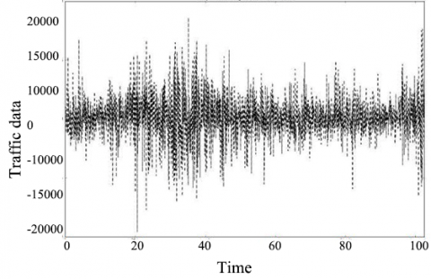
The data used in this paper are from the measured data of rapid traffic flow in four big cities in China. The specific experimental data are the measured data of four typical cities in seven elevated and fast road sections in 2018, with a total of more than 300 hours of traffic data in 50 days. After a series of filtering and processing, the time interval is 2s, and finally 221330 groups of data are obtained. The data consists of 16 sample databases, including time, city, location, weather conditions, average speed, data volume, road features and other detailed information. For convenience, 1,000 sets were intercepted from the collected data, and processed into a time series of traffic flow (Figure 1).
Figure 1. Time series of original traffic data
In this paper, the H value is estimated through wavelet analysis. First, the wavelet coefficients were obtained through discrete wavelet transform (DWT) of the time series of traffic data. Then, the spectrum of all intervals was logarithmically represented on the coordinate axes. After that, the least squares (LS) method was employed to fit a curve with slope $\Delta$ of 0.0725. The H value was derived as 0.521 to $\Delta=2 H-1$. The result obviously belongs to the interval [0.5, 1], indicating the self-similarity of the traffic data.
Since a self-similar process must have long-term correlation (LTC), it is necessary to create an LTC model to predict the traffic flow based on the self-similar traffic data. To reduce the complexity, the LTC traffic data should be decomposed into short-term correlation (STC) traffic data. Therefore, the LMD algorithm was introduced to decompose the time series of traffic data into several STC product functions (PFs). The procedure of the LMD is explained below.
First, the mean values mi of all adjacent local extremums of the original signal x(t) are connected by a straight line, and then smoothed to obtain the mean function m11(t). Then, the envelope estimation function f11(t) is obtained by the same method. Next, m11(t) is separated from the original signal x(t) to demodulate h11(t) by s11(t)=h11(t)/f11(t). These steps are repeated n times for s11(t) until s1n(t) becomes a pure frequency modulated signal. The termination condition of the iterative process can be defined as:
$\lim _{n \rightarrow \infty} f_{1 n}(t)=1$ (1)
The envelope signal can be obtained by multiplying the envelope functions:
$f_{1}(t)=\prod_{u=1}^{v} f_{1 u}(t)$ (2)
Then, the first PF of $x(t)$ is obtained as $P F_{1}(t)=f_{1}(t) s_{1 u}(t),$ and the first PF separated from $x(t)$ is taken as the new signal $w_{1}(t)$. The above process is repeated until the termination condition is realized.
Finally, the original signal $x(t)$ can be expressed as:
$x(t)=\sum_{u=1}^{k} P F_{u}(t)+w_{k}(t)$ (3)
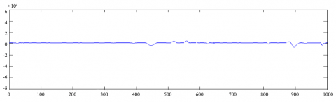
Here, the original traffic data $x(t)$ are subjected to the LMD through simulation. The termination condition was set as $1- \Delta \leq f_{1 n}(t) \leq 1+\Delta,$ where $\Delta=10^{-3} .$ The first PF $P F_{1}(t)$ was obtained after the termination condition was realized after a few iterations (Figure 1 ). Then, the second and third PFs $P F_{2}(t)$ and $P F_{3}(t)$ and the new signal $w(t)$ were collected through three more decompositions (Figure 2).
Figure 2. The PF1(t) obtained through the LMD
Figure 3. The w(t) obtained through the LMD
It can be seen that form Figure 3, the w(t) curve only oscillates slightly, and is close to the theoretical monotonic curve. The slight oscillations have no impact on the decomposition result. This means the LMD has achieved desirable effects. In other words, the LMD can convert LTC series into multiple STC PFs.
3.2 Garch-based prediction
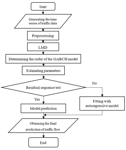
Based on the STC traffic data obtained by the LMD, the author developed a traffic flow prediction in the light of the GARCH model. As shown in Figure 4, the prediction process of the model includes the following steps.
Step $1 .$ Preprocess traffic data $S(t)$ into a time series $x(t)$.
First, the time interval $m$ was determined, and the duration $t$ of original traffic data was divided evenly into $\mu(\mu= [t / m])$ time intervals. Then, the time series $x(t): x_{1}(t), x_{2}(t), \ldots, x_{\mu}(t)$ was constructed from the traffic data in each interval.
Step 2. Decompose the time series $x(t)$.
The time series $x(t)$ was decomposed through the LMD into several PFs. The first PF was separated from the time series to obtain a new signal $w_{1}(t) .$ This process was repeated $k$ times until $w_{k}(t)$ became a monotonic function:
$\left\{\begin{aligned} w_{1}(t)=x(t)-P F_{1}(t) \\ w_{2}(t)=w_{1}(t)-P F_{2}(t) \\ \cdots \\ w_{k}(t)=w_{k-1}(t)-P F_{k}(t) \end{aligned}\right.$ (4)
Step 3. Construct the traffic flow prediction model based on the GARCH model.
Step 4. Determine the order of GARCH (r, s) by the Akaike information criterion (AIC) [20], and estimate the unknown parameters iteratively with the maximum likelihood function.
Figure 4. The prediction process of our model
Step $5 .$ Detect if the residual sequence $\left\{\varepsilon_{t}\right\}$ of $P F_{1}(t), P F_{2}(t), P F_{3}(t), \ldots P F_{n}(t), w(t)$ has white noise. If not, go to the next step; othervise, jump to Step $7 .$
Step 6. Fit the residual sequence with autoregressive model, and go to Step 3.
Step 7. Predict the traffic flow with the GARCH model.
Step 8. Add up the predicted components into the final prediction of traffic flow.
The experimental data in this paper is the measured data of a typical city, which can basically represent the flow characteristics of urban traffic flow and reflect the main factors affecting traffic flow. Therefore, using the data set for the training samples of the prediction algorithm can better train the algorithm model, it has more practical significance for the prediction results.
4.1 Simulation process
The first 1,000 sets of collected traffic data were used to train our model, and the remaining data were compared with the prediction results of the model. As mentioned before, the self-similarity test and the LMD of the original data have been completed. Thus, this section only needs to obtain the PFs through the LMD and predict the traffic flow by the GARCH model.
Before prediction, the author tested if the residual sequence of each PF is heteroscedastic through Portmanteau Q-test and Lagrange multiplier (LM) test. The test results of $P F_{1}(t)$ are recorded in Table 1 below.
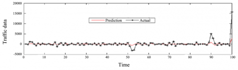
As shown in Table 1, both test results indicate that residual sequence of $P F_{1}(t)$ had conditional heteroscedasticity before the 12th order. Similarly, the residual sequences of the other PFs were proved to be heteroscedastic. Hence, the GARCH model is suitable for predicting the traffic flow. The prediction results are compared with the actual data as Figure 5.
It can be seen from Figure 5 that the prediction results only had slight deviations from the actual data, revealing the accuracy of our model. To evaluate the prediction results more objectively, the root means square error (RMSE) and relative root mean square error (RRMSE) were taken as the evaluation criteria:
Table 1. Heteroscedasticity of the residual sequence of $P F_{1}(t)$
|
Order |
1 |
2 |
3 |
4 |
5 |
6 |
7 |
8 |
9 |
10 |
11 |
12 |
|
Q |
45.98 |
66.07 |
88.72 |
97.82 |
101.85 |
103.81 |
106.77 |
107.17 |
107.19 |
107.28 |
107.51 |
107.64 |
|
p>Q |
<.0001 |
<.0001 |
<.0001 |
<.0001 |
<.0001 |
<.0001 |
<.0001 |
<.0001 |
<.0001 |
<.0001 |
<.0001 |
<.0001 |
|
LM |
45.11 |
45.92 |
51.78 |
52.59 |
52.30 |
53.01 |
53.17 |
54.37 |
54.37 |
54.82 |
54.85 |
54.88 |
|
p>LM |
<.0001 |
<.0001 |
<.0001 |
<.0001 |
<.0001 |
<.0001 |
<.0001 |
<.0001 |
<.0001 |
<.0001 |
<.0001 |
<.0001 |
Figure 5. The prediction results of the GARCH model
$R M S E=\sqrt{\frac{1}{N} \sum_{t=1}^{N}\left(x(t)-x^{\prime}(t)\right)^{2}}$ (5)
$R R M S E=\sqrt{\frac{1}{N} \sum_{t=1}^{N}\left(\frac{x(t)-x^{\prime}(t)}{x(t)}\right)^{2}}$ (6)
where, N is the number of predicted traffic data sets; $x^{\prime}(t)$ is the predicted traffic flow at the t-th moment; $x(t)$ is the actual traffic flow at the t-th moment. The RMSE and RRMSE of each PF are listed in Table 2.
Table 2. The RMSE and RRMSE of Each PF
|
|
$P F_{1}(t)$ |
$P F_{2}(t)$ |
$P F_{3}(t)$ |
w(t) |
|
RMSE |
7.58×10² |
6.33×10² |
4.01×10² |
1.12×10² |
|
RRMSE |
11.823 |
7.592 |
5.891 |
5.149 |
As shown in Table 2, both the RMSE and RRMSE declined with the increase in the order of the PF, an evidence of the gradually improving prediction accuracy. In addition, $P F_{1}$ had the largest RMSE and RRMSE among all PFs, i.e. the lowest prediction accuracy. Thus, the accuracy of our model can be further enhanced by improving the prediction accuracy of $P F_{1}$. This calls for detailed analysis on the signal features of this PF.
In the GARCH model, the regression function cannot extract all the relevant information from the residual sequence, if the latter is autocorrelated rather than completely stochastic. In this case, the GARCH model should be improved by fitting the residual sequence with the autoregressive model.
According to the Durbin–Watson (DW) test results on the improved GARCH model, the value of p<DW was less than 0.0001 when testing the autocorrelation of the 5th order delay of $P F_{1}$ ’s residual sequence. This means the residual sequence of $P F_{1}$ has significant positive correlation. Therefore, the improved model is suitable for traffic flow prediction. The predicted results are shown in Figure 6 below.
Figure 6. The prediction results of improved GARCH model
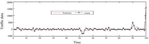
As shown in Figure 6, the improved GARCH model predicted burst traffic well with an RMSE of 6.69×10² and an RRMSE of 8.138. The prediction accuracy was obviously higher than that of the original GARCH model.
4.2 Comparative Analysis
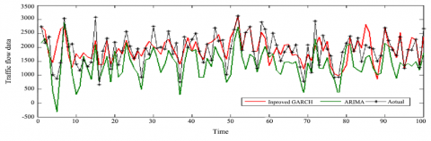
The final prediction of the traffic flow $x^{\prime}(t)$ was obtained by adding up the predicted values of the PFs. Then, the predicted results of our model (improved GARCH) were compared with those of the GARCH model, the ARIMA model and the improved ARIMA [20-21] (Figures 7 and 8, Table 3).
Figures 7 and 8 show that our model outperformed the GARCH and the ARIMA in the prediction of traffic flow. The data in Table 3 demonstrate that the prediction accuracy of our model was higher than the two contrastive models. Overall, the results fully manifest the feasibility of our model for traffic flow prediction.
Figure 7. Comparison between our model and the GARCH model
Figure 8. Comparison between our model and the ARIMA model
Table 3. Comparison Between Our Model, GARCH Model, ARIMA and IMPROVED ARIMA Model
|
|
RMSE |
RRMSE |
|
Our model |
4.38×10² |
0.332 |
|
GARCH model |
6.11×10² |
0.347 |
|
ARIMA model |
6.25×10² |
0.387 |
|
Improved ARIMA model |
6.01×10² |
0.341 |
In this paper, the traffic data collected from four big cities in China are proved to be self-similar through the analysis of traffic flow features. Thus, the traffic flow should be forecasted with a model with self-similarity. To simplify the model and enhance prediction accuracy, the LTC time series of traffic data were decomposed into STC PFs through the LMD. On this basis, a traffic prediction model was developed based on the LMD and the GARCH model. Then, the proposed model was compared with the original GARCH model, ARIMA model and improved ARIMA model through simulation. The comparison results showed that our model outperformed the contrastive models in prediction accuracy. Thus, our model improved the prediction accuracy of traffic flow greatly. With the continuous research and development of big data and flow prediction algorithm, the accuracy of prediction algorithm needs to be further improved in view of the diversity of traffic flow data and the change of practical application scenarios, it will be our research focus in the future.
The project supported by the Scientific Searching Plan Project of Shaanxi Province. Education Department (No.: 16JK1184), and the colleges and universities study innovation fund supported by science and technology development center of the ministry of education (No.: 2018A03024). Authors are grateful to the related departments for the financial supports to carry out this work.
[1] Lv, Y.S., Duan, Y.J., Kang, W.W., Li, Z.X., Wang, F.Y. (2015). Traffic flow prediction with big data: A deep learning approach. IEEE Transactions on Intelligent Transportation Systems, 16(2): 865-873. https://doi.org/10.1109/TITS.2014.2345663
[2] Wei, G.Y., Ling, Y., Guo, B.F., Xiao, B., Vasilakos, A.V. (2011). Prediction-based data aggregation in wireless sensor networks: Combining grey model and Kalman Filter. Computer Communications, 34(6): 793-802. https://doi.org/10.1016/j.comcom.2010.10.003
[3] Golestan, S., Guerrero, J.M., Vasquez, J.C. (2018). Steady-state linear Kalman filter-based plls for power applications: A second look. IEEE Transactions on Industrial Electronics, 65(12), 8331945: 9795-9800. https://doi.org/10.1109/TIE.2018.2823668
[4] Ahmed, S.A., Cook, A.R. (1982). Discrete dynamic models for freeway incident detection systems. Transportation Planning & Technology, 7(4): 231-242. https://doi.org/10.1080/03081068208717226
[5] Ghosh, B., Basu, B., O'Mahony, M. (2009). Multivariate short-term traffic flow forecasting using time-series analysis. IEEE Transactions on Intelligent Transportation Systems, 10(2): 246-254. https://doi.org/10.1109/TITS.2009.2021448
[6] Yang, Z.S., Bing, Q., Zhou, Q.C., Lin, C.Y., Yang, N., Mei, D. (2014). Research on short-term traffic flow prediction method based on similarity search of time series. Journal of Transport Information & Safety, 2014(7): 1-8. http://dx.doi.org/10.1155/2014/184632
[7] Muruganantham, A., Zhao, Y., Gee, S.B., Qiu, X., Tan, K.C. (2013). Dynamic multiobjective optimization using evolutionary algorithm with Kalman filter. Procedia Computer Science, 24(1): 66-75. https://doi.org/10.1016/j.procs.2013.10.028
[8] Huang, M.L. (2015). Intersection traffic flow forecasting based on ν-GSVR with a new hybrid evolutionary algorithm. Neurocomputing, 147(1): 343-349. https://doi.org/10.1016/j.neucom.2014.06.054
[9] Csikós, A., Varga, I., Hangos, K.M. (2018). A hybrid model predictive control for traffic flow stabilization and pollution reduction of freeways. Transportation Research Part D: Transport and Environment, 59: 174-191. https://doi.org/10.1016/j.trd.2018.01.006
[10] Iwamura, Y., Tanimoto, J. (2018). Complex traffic flow that allows as well as hampers lane-changing intrinsically contains social-dilemma structures. Journal of Statistical Mechanics: Theory and Experiment, 2018(2): 023408. https://doi.org/10.1088/1742-5468/aaa8ff
[11] Kumar, S.V., Vanajakshi, L. (2015). Short-term traffic flow prediction using seasonal ARIMA model with limited input data. European Transport Research Review, 7(3): 21-28. https://doi.org/10.1007/s12544-015-0170-8
[12] Jin, S., Wang, D.H., Xu, C., Ma, D.F. (2013). Short-term traffic safety forecasting using Gaussian mixture model and Kalman filter. Journal of Zhejiang University - Science A: Applied Physics & Engineering, 14(4): 231-243. https://doi.org/10.1631/jzus.A1200218
[13] Hanifelou, Z., Adibi, P., Monadjemi, S.A., Karshenas, H. (2018). KNN-based multi-label twin support vector machine with priority of labels. Neurocomputing, 322: 177-186. https://doi.org/10.1016/j.neucom.2018.09.044
[14] Huan, J. (2015). Research on automobile engine failure recognition technology based on improved PSO-RVM algorithm. Applied Mechanics and Materials, 727-728: 757-760. https://doi.org/10.4028/www.scientific.net/AMM.727-728.757
[15] Yao, Z.H., Jiang, Y.S., Han, P., Luo, X.L., Xu, T. (2017). Traffic flow prediction model based on neural network in small time granularity. Journal of Transportation Systems Engineering & Information Technology, 17(1): 67-73. https://doi.org/10.16097/j.cnki.1009-6744.2017.01.011
[16] Guo, Y., Lu, L. (2018). Application of a traffic flow prediction model based on neural network in intelligent vehicle management. International Journal of Pattern Recognition & Artificial Intelligence, S0218001419590092. https://doi.org/10.1142/S0218001419590092
[17] Othman, S.M., Ba-Alwi, F.M., Alsohybe, N.T., Al-Hashida, A.Y. (2018). Intrusion detection model using machine learning algorithm on Big Data environment, Journal of Big Data, 5(1): 34. https://doi.org/10.1186/s40537-018-0145-4
[18] Wu, Y., Tan, H.C., Qin, L.Q., Ran, B., Jiang, Z.X. (2018). A hybrid deep learning-based traffic flow prediction method and its understanding. Transportation Research Part C Emerging Technologies, 90: 166-180. https://doi.org/10.1016/j.trc.2018.03.001
[19] Lv, Y.S., Duan, Y.J., Kang, W.W. (2007). Traffic flow prediction with big data: A deep learning approach. IEEE Transactions on Intelligent Transportation Systems, 16(2): 865-873. https://doi.org/10.1109/TITS.2014.2345663
[20] Seghouane, A.K., Amari, S.I. (2007). The AIC criterion and symmetrizing the Kullback–Leibler divergence. IEEE Trans Neural Netw, 18(1): 97-106. https://doi.org/10.1109/TNN.2006.882813
[21] Kumar, S.V., Vanajakshi, L. (2015). Short-term traffic flow prediction using seasonal ARIMA model with limited input data. European Transport Research Review, 7(3): 21-33. https://doi.org/10.1007/s12544-015-0170-8