Leixiao Li | Jing Gao* | Hui Wang | Dan Deng | Hao Lin
OPEN ACCESS
This paper probes into the all-to-all comparison of large dataset, and gives a formal mathematical description of the problem. Then, a multi-objective file distribution model was constructed based on the LP, aiming to localize the data, balance node storage and loads, minimize the storage occupation, and control the occupied storage within the storage limit of each node. To save storage space, the established model was further optimized, and the file distribution algorithm was designed for the distributed environment. Experimental results show that our model and algorithm successfully balanced the storage occupation and loads between computing nodes, and minimized the occupation of node storage.
distributed system, all-to-all comparison problem, file distribution, linear programming (LP), model optimization
All-to-all comparison of big dataset, a commonplace in bioinformatics, biometrics and data mining, is a special computing problem that compares and computes any two files in a dataset [1]. Distributed computing with distributed storage is often adopted to solve the problem, due to its high efficiency, reliability and scalability. This method breaks down a large problem into multiple small ones, and processes each of them at separate nodes in the distributed system [2]. The effect of distributed computing depends heavily on the strategies of data distribution, task decomposition and task scheduling. The computing performance may not be desirable if the comparison task faces the following problems: the data are distributed irrationally, the data are not highly localized, and the loads are imbalanced in the distributed system [3].
The existing solutions to all-to-all comparison of big dataset fall into two categories: the centralized computing and distributed computing with centralized storage [4]. The latter often encounters problems like task delay, owing to the limited storage and the wait for data transfer [5]. Therefore, some scholars have applied distributed computing with distributed storage in all-to-all comparison of big dataset. This method offers two data allocation strategies: assigning each input file to a computing node, and distributing several duplicates of each input file randomly to system nodes (the Hadoop distribution strategy) [6-8]. The first strategy has similar problems with centralized computing, which also stores all input files on every system node [9]. Under the Hadoop distribution strategy [10], the huge amount of data exchange between the nodes will drag down computing efficiency. After all, the Hadoop distribution strategy is an all-purpose framework, not specifically designed for all-to-all comparison [11-13].
To solve the problems in the solutions to all-to-all comparison of big dataset, this paper formally describes the problem of all-to-all comparison of big dataset, sets up a constrained optimization model for file distribution, and designs a file distribution algorithm based on linear programming (LP). Next, the proposed model and algorithm were verified through experiments under the constraints on data localization and node storage in distributed system. The experimental results show that our model and algorithm successfully balanced the loads between computing nodes, minimized the occupation of node storage, and minimized the load in a cluster environment. The research findings greatly improve the overall performance of the distributed cluster environment, giving full play to the advantages of distributed system.
All-to-all comparison refers to the pairwise comparison between all items in the target dataset. Let A={A1, A2, A3, ......, Am} be the target dataset, C be the comparison function that computes the items in the dataset, and M be the similarity matrix of the results. Then, the all-to-all comparison can be described as:
$\mathrm{M}_{\mathrm{ij}}=\mathrm{C}\left(A_{i}, A_{j}\right)=\mathrm{C}\left(A_{j}, A_{i}\right), i, j=1,2, \ldots \ldots, m$ (1)
where Ai is the i-th item in A; Mij is an element of M, i.e. the result of the comparison between Ai and Ai; m is the number of items in A.
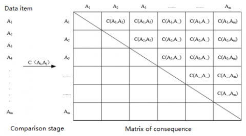
Figure 1 presents a typical all-to-all comparison problem, in which each item should be compared with all the other items. In the matrix shown in Figure 1, the pairwise comparisons, e.g. C(Ai, Aj)=C(Aj, Ai), are all unordered. Since the matrix is symmetric, only the upper triangular elements need to be considered in the typical all-to-all comparison problem.
Figure 1. A typical problem of all-to-all comparison
In a distributed cluster environment, the all-to-all comparison of a big dataset means the pairwise comparison between all the data files in the dataset. Before pairwise comparison, all the data files should be distributed to the computing nodes of the distributed system. The file distribution should give full consideration of how system computing performance is affected by the following factors: file localization, load balance, mean load of nodes, node storage, data transmission and network bandwidth.
The file distribution must satisfy the following conditions to ensure the overall computing performance of the distributed system:
(1) The data files should be localized for comparison, i.e. the two files to be compared on a node must be saved on that node.
(2) The comparison tasks should be assigned unevenly across the computing nodes.
(3) The data distributed to each node should be balanced, within the storage limit of the node and occupy the least possible storage.
The above description shows that the all-to-all comparison problem is a typical constraint optimization problem. In this paper, the optimization aims to balance the comparison tasks of the computing nodes, under the constraints of data localization, balanced data distribution and minimal occupation of node storage, thereby speeding up comparison speed and overall system performance.
Constrained optimization problem attempts to maximize or minimize the value of the objective function under multiple constraints. The most effective solution to constrained optimization is the LP, which requires that objective function and all constraints are linear [14, 15]. The main goal of the LP is to find the control sequence that minimizes the value of the objective function under all constraints. The LP can also effectively solve control and planning problems, thanks to its strong modelling abilities [16].
Taking the balancing of node loads as the objective, the file distribution of the all-to-all comparison problem was modeled under the constraints of the problem and the constraints on node storage. The constraints were expressed as equality or inequality.
Let m be the number of genetic sequence files and n be the number of nodes in a distributed system. These data files need to be distributed to the nodes for pairwise comparison. The node loads should be balanced under two constraints: the data should be localized, and the size of the distributed file should not exceed the node storage.
As shown in Figure 2, the total number of pairwise comparisons for the m data files can be obtained as:
$C_{m}^{2}=\frac{m(m-1)}{2}$ (2)
Let si (i=1, 2, ⋯, m) be the size of each data file. Then, the total size of the two files in each pairwise comparison can be computed as:
$w_{i j}=s_{i}+s_{j}\left(i, j=1,2 \cdots, m, i<j\right)$ (3)
The load of the pairwise comparison between files i and j can be computed as:
$c_{i j}\left(i, j=1,2, \cdots, m,i<j\right)$ (4)
Thus, the total number of pairwise comparisons between the m data files can be described as:
$\sum_{i=1}^{m} \sum_{j=i+1}^{m} c_{ij}$ (5)
If the pairwise comparison tasks are distributed equally to n nodes, then the theoretical mean number of tasks allocated to each node can be expressed as:
$\frac{\sum_{i=1}^{m} \sum_{j=i+1}^{m} c_{i j}}{n}$ (6)
Then, $x_{k t}\left(k=1,2, \cdots, \frac{m(m-1)}{2}, t=1,2, \cdots, n\right)$ was introduced to specify the k-th pairwise comparison task is allocated to node n:
$x_{k t}=0 or 1, \quad k=1,2, \cdots, \frac{m(m-1)}{2}, t=1,2, \cdots, n$ (7)
Since each task can only be allocated to one node, we have:
$\sum_{t=1}^{n} x_{k t}=1, k=1,2, \cdots, \frac{m(m-1)}{2}$ (8)
Let uj (j=1, 2, ⋯, n) be the storage limit of node n and Wkt=wijt be the total size of the files i and j in the k-th task distributed to node t. Then, the constraint that the the total size of the files distributed to each node in the distributed system should not exceed the storage limit of that node can be expressed as:
$\sum_{k=1}^{\frac{m(m-1)}{2}} \mathrm{W}_{kt} x_{k t} \leq u_{t}, t=1,2, \cdots, n$ (9)
Let Ckt=cijt be the load of the k-th task between files i and j allocated to node t. Then, the load of the task distributed to a node in the distributed system can be expressed as:
${\sum_{k=1}^{\frac{m(m-1)}{2}}} \mathrm{C}_{k t} x_{k t}$ (10)
Then, the sum of the absolute difference between the actual and theoretical mean loads of the task distributed to each node in the distributed system can be described as:
$\sum_{t=1}^{n}\left|\left(\sum_{k=1}^{\frac{m(m-1)}{2}} \mathrm{C}_{k t} x_{k t}\right)-\frac{\sum_{i=1}^{m} \sum_{j=i+1}^{\mathrm{m}} c_{i j}}{n}\right|$ (11)
Taking (6)~(8) as the constraints, the file distribution model can be established to minimize the value of Eq. (12):
$ \min \sum\limits_{t=1}^{n}{|(\sum\limits_{k=1}^{\frac{m(m-1)}{2}}{{{\text{C}}_{kt}}{{x}_{kt}})-\frac{\sum\limits_{i=1}^{m}{\sum\limits_{j=i+1}^{\text{m}}{{{c}_{ij}}}}}{n}}|} $
$ s.t.\left\{ \begin{align} & \sum\limits_{t=1}^{n}{x{}_{kt}=1},k=1,2,\cdots ,\frac{m(m-1)}{2} \\ & \sum\limits_{k=1}^{\frac{m(m-1)}{2}}{{{\text{W}}_{kt}}{{x}_{kt}}}\le {{u}_{t}},t=1,2,\cdots ,n \\ & x{}_{kt}=0\text{ }or\text{ 1}k=1,2,\cdots ,\frac{m(m-1)}{2},t=1,2,\cdots ,n \\ \end{align} \right. \\ $(12)
If the objective function in Eq. (12) contains nonlinear terms, then established model is a nonlinear programming model. In this case, new decision variables $d_{t}^{-}$ and $d_{t}^{+}$ were introduced to transform Equation (12) into a linear model. The two variables are both numbers greater than or equal to zero. The former means the load allocated to node t exceeds the theoretical mean load, and the latter has the exactly opposite meaning. In the former case, the excess load $d_{t}^{-}$ should be removed from the node, changing the objective into searching for the minimum value of $\left(d_{t}^{-}+d_{t}^{+}\right)$ for each node. In the latter case, the insufficient load $d_{t}^{+}$ should be added to the node.
With the addition of the new decision variables, Equation (12) can be transformed into the LP model below:
$\min \sum\limits_{t=1}^{n}{(d_{t}^{-}+d_{t}^{+}}) $
$s.t.\left\{ \begin{align} & \sum\limits_{t=1}^{n}{x{}_{kt}=1},k=1,2,\cdots ,\frac{m(m-1)}{2} \\ & \sum\limits_{k=1}^{\frac{m(m-1)}{2}}{{{\text{W}}_{kt}}{{x}_{kt}}}\le {{u}_{t}},t=1,2,\cdots ,n \\ & ((\sum\limits_{k=1}^{\frac{m(m-1)}{2}}{{{\text{C}}_{kt}}{{x}_{kt}})-\frac{\sum\limits_{i=1}^{m}{\sum\limits_{j=i+1}^{\text{m}}{{{c}_{ij}}}}}{n}})-d_{t}^{-}+d_{t}^{+}=0,t=1,2,\cdots ,n \\ & x{}_{kt}=0\text{ }or\text{ 1}k=1,2,\cdots ,\frac{m(m-1)}{2},t=1,2,\cdots ,n \\ & d_{t}^{-},d_{t}^{+}\ge 0,t=1,2,\cdots ,n \\ \end{align} \right. \\ $ (13)
Since neither $d_{t}^{-}$ and $d_{t}^{+}$ are integers, Eq. (13) is a mixed integer linear programming (MILP) model.
By the MILP model, the node loads in the distributed environment can be basically balanced, but the files allocated to each node still take up much of the node storage (Section 6). The node storage of the model should be further reduced.
The load allocated to each node in the cluster environment can be computed by the MILP model. It is assumed that the cumulative load of each node obtained by the MILP is:
$C_{j}(j=1,2, \cdots, n)$ (14)
Assuming that Cmax=max{C1, C2, ..., Cn}, two decision variables were introduced, namely, yrt(r=1, 2, ..., m, t=1, 2, ..., n) and xkt. The former specifies if the r-th file to be compared is stored in node t, and the latter specifies if the files of the k-th pairwise comparison are stored in node t.
If xkt=1, both files of the k-th pairwise comparison are be stored in node t. Then, the total storage of each node in the distributed environment can be expressed as:
$\sum_{r=1}^{m} \sum_{t=1}^{n} s_{r} y_{r t}$ (15)
The relationship between the two decision variables can be described as:
$\sum_{k \in U_{r}} x_{k t} \leq n y_{r t}(r=1,2, \cdots, m, t=1,2, \cdots, n)$ (16)
where Ur is the set of all sequence number k containing the r-th file. Obviously, yrt=1 if at least one element of $x_{k t}\left(k \in U_{r}\right)$ equals 1.
According to (12), (14) and (15), the optimized MILP model can be established to minimize the total storage of all nodes in the distributed environment:
$ \min \sum\limits_{r=1}^{m}{\sum\limits_{t=1}^{n}{{{s}_{r}}{{y}_{rt}}}} $
$ s.t.\left\{ \begin{align} & \sum\limits_{t=1}^{n}{x{}_{kt}=1},k=1,2,\cdots ,\frac{m(m-1)}{2} \\ & \sum\limits_{k=1}^{\frac{m(m-1)}{2}}{{{c}_{kt}}{{x}_{kt}}}\le {{C}_{\max }},t=1,2,\cdots ,n \\ & \sum\limits_{k\in {{U}_{r}}}{{{x}_{kt}}\le n{{y}_{rt}}}(r=1,2,\cdots ,m,t=1,2,\cdots ,n) \\ & x{}_{kt}=0\text{ }or\text{ 1}k=1,2,\cdots ,\frac{m(m-1)}{2},t=1,2,\cdots ,n \\ & {{y}_{rt}}=0\text{ }or\text{ 1}r=1,2,\cdots ,m,t=1,2,\cdots ,n \\ \end{align} \right. \\ $ (17)
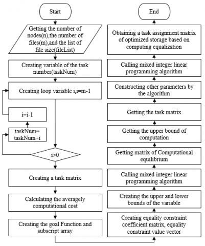
The optimized MILP model is divided into two phases: computing the matrix of file distribution results, and minimizing the total storage of all nodes under load balancing. The flow chart of the algorithm is shown in Figure 2.
Figure 2. Flow chart of file distribution algorithm
To validate the established model and algorithm, the following four file distribution experiments were conducted on Matlab 2018a.
6.1 Same file size and equal distribution of tasks
Ten genetic sequence files of the same size (1MB) were distributed to five nodes for sequence alignment. As shown in Figure 3, the nodes were given the same task load, a sign of full load balancing.
Figure 3. Load distribution in the first experiment
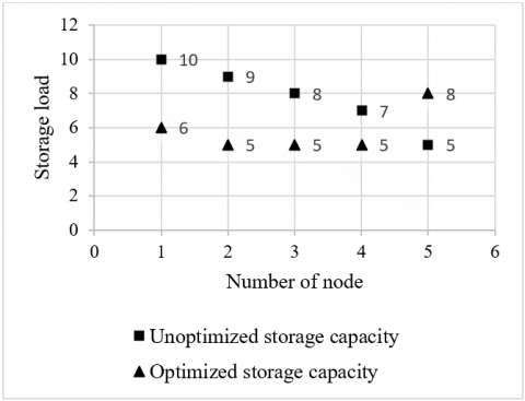
Figure 4 shows the variation in the node storage required to store the distributed files through model optimization. It can be seen that, due to the model optimization, 4M storage was saved on node 1, 4M on node 2, 3M on node 3, 2M on node 4, and 3M more was occupied on node 5. Overall, the five nodes in total saved 10M of storage, and the node storages were basically balanced after the optimization.
Figure 4. The variation in the node storage required to store the distributed files through model optimization in the first experiment
6.2 Same file size and unequal distribution of tasks
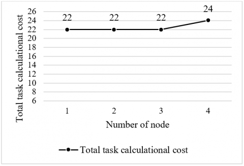
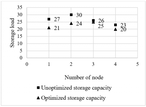
Ten genetic sequence files of the same size (1MB) were distributed to four nodes for sequence alignment. Since m=10 and n=4 and the files are of the same size, we have $m(m-1) \%(2 * n) \neq 0$, that is, the nodes cannot achieve complete load balance. As shown in Figure 5, three of the four nodes were respectively given 22 tasks, and the remaining one was given 24 tasks. The nodes basically achieved load balance.
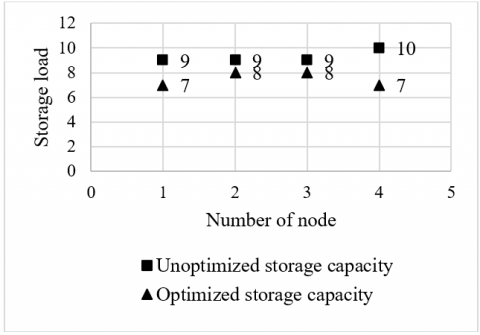
Figure 6 shows the variation in the node storage required to store the distributed files through model optimization. It can be seen that, due to the model optimization, 2M storage was saved on node 1, 1M on node 2, 1M on node 3, and 3M on node 4. Overall, the four nodes in total saved 7M in storage and the node storages were basically balanced after the optimization.
Figure 5. Load distribution in the second experiment
Figure 6. The variation in the node storage required to store the distributed files through model optimization in the second experiment
6.3 Different file sizes and equal distribution of tasks
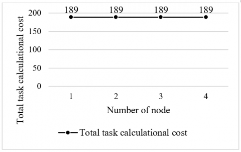
Eight genetic sequence files of different sizes (15MB; 12MB; 5MB; 7MB; 1MB; 6MB; 35MB; 27MB) were allocated to four nodes for sequence alignment. Since m=8 and n=4, we have $m(m-1) \%(2 * n)=0$. However, the nodes may not be able to achieve complete load balance, owing to the difference in file size. As shown in Figure 7, the four nodes were each given 189 tasks, reaching complete load balance.
Figure 7. Load distribution in the third experiment
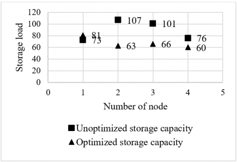
Figure 8. The variation in the node storage required to store the distributed files through model optimization in the third experiment
Figure 8 shows the variation in the node storage required to store the distributed files through model optimization. It can be seen that, due to the model optimization, 8M more storage was occupied on node 1, 44M storage was saved on node 2, 35M on node 3, and 16M on node 4. Overall, the four nodes in total saved 87M in storage and the node storages were basically balanced after the optimization.
6.4 Different file sizes and unequal distribution of tasks
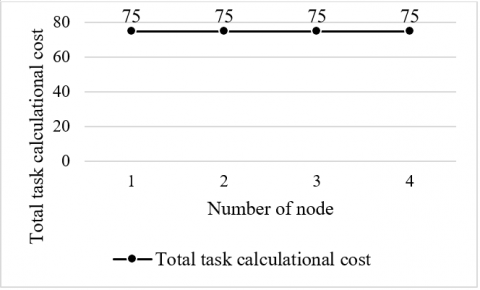
Eleven genetic sequence files of different sizes (2MB; 1MB; 1MB; 5MB; 4MB; 2MB; 5MB; 1MB; 3MB; 2MB; 4MB) were allocated to four nodes for sequence alignment. As shown in Figure 9, the four nodes were each given 75 tasks, reaching complete load balance.
Figure 10 shows the variation in the node storage required to store the distributed files through model optimization. It can be seen that, due to the model optimization, 6M more storage was occupied on node 1, 6M storage was saved on node 2, 7M on node 3, and 3M on node 4. Overall, the four nodes in total saved 16M in storage and the node storages were basically balanced after the optimization.
Figure 9. Load distribution in the fourth experiment
Figure 10. The variation in the node storage required to store the distributed files through model optimization in the fourth experiment
The four experiments demonstrate that, if load balance is theoretically possible, the node loads were always fully balanced, whether the file sizes are the same or not, under the following two constraints: the data are fully localized, and the files distributed to a node do not surpass the storage limit of that node. Even if load balance is theoretically impossible, our model and algorithm could minimize the load difference between nodes and achieve basically the load balance.
The optimized model further reduced the overall storage pressure. According to the variation in the node storage observed in each experiment, the model optimization greatly lowered the node storage required to save the distributed files.
This paper probes into the all-to-all comparison of large dataset, and gives a formal mathematical description of the problem. Then, a multi-objective file distribution model was constructed based on the LP, aiming to localize the data, balance node storage and loads, minimize the storage occupation, and control the occupied storage within the storage limit of each node. To save storage space, the established model was further optimized, and the file distribution algorithm was designed for the distributed environment. Finally, our model and algorithm were proved valid through several experiments.
The work is funded in part by the National Natural Science Foundation of China (NSFC) under Grant No. 61462070, the Doctoral research fund project of Inner Mongolia Agricultural University under Grant No. BJ09-44 and the Inner Mongolia Autonomous Region Key Laboratory of big data research and application for agriculture and animal husbandry.
[1] Zhang, Y.F., Tian, Y.C., Kelly, W., Fidge, C., Gao, J. (2015). Application of simulated annealing to data distribution for all-to-all comparison problems in homogeneous systems. International Conference on Neural Information Processing, Springer, Cham, 683-691. https://doi.org/10.1007/978-3-319-26555-1_77
[2] Baert, Q., Caron, A.C., Morge, M., Routier, J.C. (2018). Fair task allocation for large data sets analysis. Revue d'Intelligence Artificielle, 31(4): 401-426. https://doi.org/10.3166/RIA.31.401-426
[3] Zhang, Y.F., Tian, Y.C., Kelly, W., Fidge, C. (2014). A distributed computing framework for all to all comparison problems. Proceedings of IECON’14. Washington D. C, USA: IEEE Press, 2499-2505. https://doi.org/10.1109/IECON.2014.7048857
[4] Li, L.X., Gao, J., Mu, R. (2019). Optimal data file allocation for all-to-all comparison in distributed system: A case study on genetic sequence comparison. International Journal of Computers, Communications & Control, 14(2): 199-211. https://doi.org/10.15837/ijccc.2019.2.3526
[5] Shen, X., Choudhary, A. (2003). A distributed multi-storage resource architecture and I/O performance prediction for scientific computing. Cluster Computing, 6(3): 189-200. https://doi.org/10.1109/HPDC.2000.868631
[6] Song, A., Zhao, M., Xue, Y., Luo, J. (2016). MHDFS: A memory-based hadoop framework for large data storage. Scientific Programming, 2016: 1808396. http://dx.doi.org/10.1155/2016/1808396
[7] Chen, F., Liu, J., Zhu, Y. (2017). A real-time scheduling strategy based on processing framework of hadoop. 2017 IEEE International Congress on Big Data (BigData Congress), 2017: 321-328. https://doi.org/10.1109/BigDataCongress.2017.48
[8] Lin, W. (2012). An improved data placement strategy for Hadoop. Journal of South China University of Technology (Natural Science Edition), 40(1): 152-158.
[9] Li, X., Zhang, H., Hu, Q., Huang, X. (2017). Research on power customer segmentation based on big data of intelligent city. 2017 29th Chinese Control and Decision Conference (CCDC), 3207-3211. http://dx.doi.org/10.1109/CCDC.2017.7979059
[10] Ghemawat, S., Gobioff, H., Leung, S.T. (2003). The google file system.
[11] Lin, X., Lin, P., Huang, P., Chen, L., Fan, Z., Huang, P. (2015). Modeling the task of google mapreduce workload. 2015 15th IEEE/ACM International Symposium on Cluster, Cloud and Grid Computing, 1229-1232. https://doi.org/10.1109/CCGrid.2015.104
[12] Guo, Y., Rao, J., Cheng, D., Zhou, X. (2016). iShuffle: Improving hadoop performance with shuffle-on-write. IEEE Transactions on Parallel and Distributed Systems, 28(6): 1649-1662. https://doi.org/10.1109/TPDS.2016.2587645
[13] Jiao, X., Mu, J., He, Y.C., Chen, C. (2017). Efficient ADMM decoding of LDPC codes using lookup tables. IEEE Transactions on Communications, 65(4): 1425-1437. https://doi.org/10.1109/TCOMM.2017.2659733
[14] Qin, Z., Liu, X., Cao, B. (2016). Multi-level linear programming subject to max-product fuzzy relation equalities. International workshop on Mathematics and Decision Science, Springer, Cham, 220-226. https://doi.org/10.1007/978-3-319-66514-6_23
[15] Sinha, S.B., Sinha, S. (2004). A linear programming approach for linear multi-level programming problems. Journal of the Operational Research Society, 55(3): 312-316. https://doi.org/10.1057/palgrave.jors.2601701
[16] El-Bakry, M. (2010). Using linear programming models for minimizing harmonics values in cascaded multilevel inverters. 2010 IEEE/ASME International Conference on Advanced Intelligent Mechatronics, 696-702. https://doi.org/10.1109/AIM.2010.5695713