Tingting Lei | Guangtian Zou*
OPEN ACCESS
The commercial space signage system (CSSS) both presents the information of the commercial building and promotes the exposure of certain brands. Thus, the CSSS design is the key to the design of the commercial building, exerting a direct impact on consumer experience in the building. However, there is no unified or effective method to quantify the effect of the CSSS design. To make up for this gap, this paper puts forward an interactive method to analyze and evaluate the CSSS design based on object detection. With the aid of the virtual reality (VR) technology, the author constructed an object detection model based on the Residual Network (ResNet), and used it to simulate the visual experience of the user walking through the commercial space. The generated visual data were analyzed with several indices on significance and discrimination. The comparative experiments show that the analysis results of our method agree well with the actual visual experience, indicating that our method can effectively quantify the effect of the CSSS design. The research findings shed new light on the optimization of the CSSS design.
commercial space signage system (CSSS), interactive design, object detection, analysis and evaluation, convolutional neural network (CNN)
The global shift towards a more urban population has sparked a growth in the number of commercial buildings. In large commercial buildings, the interior decoration is updated rapidly, and the spatial layout is becoming increasingly complex. These trends highlight the importance of interior signage system to commercial buildings. The demand for signage system gradually increases, as today’s large commercial buildings tend to integrate complex functions and spaces. The composite design makes it imperative to improve the shopping experience through the provision of effective information.
In the commercial space, a good signage system should meet the basic behavioral needs (e.g. consumption and travel) of the user, and provide them with impressive, visual information that are reliable and trustworthy. The information provision must be quick, efficient and orderly, laying the psychological basis for the user and making consumption behavior more orderly [1]. Therefore, it is very meaningful to develop a method that analyzes and evaluates whether a signage system can provide clear guidance to the user.
Traditionally, the commercial space signage system (CSSS) was designed based on various factors, namely, the type of building, environment, landscape coordination and investment risk. Many of these factors are difficult to be analyzed theoretically or quantified accurately. What is worse, the architectural designs are often presented and demonstrated unintuitively. This calls for a visual and realistic technology to demonstrate these designs [2].
In the design phase, the effect of the CSSS is generally analyzed and evaluated subjectively, without any unified quantification method. In fact, the design of signage system should not be purely static. The consumption behavior is dynamic in large commercial buildings, so it is with the search for environmental information. Therefore, the signage system for a large commercial building must be designed based on the actual experience of the user, such as the viewing distance, travel direction and color changes. These elements pose different requirements on the design of the signage system [3].
The major role of the CSSS is to provide information to the user. The effect of signage design can be directly and effectively analyzed from the perspective of vision, which is the most important way for human to receive and perceive external information. After all, human relies on vision to receive 87 % of external information and perform 76~90 % of activities [4]. In addition, the signage system should stand out from the surroundings in large commercial buildings, enabling the user to identify the signs easily and perceive the information on the signs without disturbing their commercial behavior. Thus, it is possible to measure the interactivity and effectiveness of the CSSS by the significance of signs and the discrimination between different types of signs.
Both significance and discrimination can be quantified based on the field of view (FOV) image of the user walking through the commercial space. Meanwhile, the user’s observation behavior can be simulated effectively with the object detection technology in computer vision. The convolutional neural network (CNN), a deep learning method, has been a popular way to process and analyze the FOV images. Because of its local receptive fields, the CNN is robust to scale changes [5], and thus able to capture the geometric information (e.g. position) of the object. The excellence of the network has been proved through extensive applications in image testing [6-7].
In the CNN, the flexible convolutional blocks [8] and the pooling layer [9] are inspired by two classic concepts in visual neuroscience: simple cells and complex cells [10]. The network replicates known basic visual functions of primates, and operates on an architecture mimicking the LGN-V1-V2-V4-IT structure of the ventral visual pathway. Reference [11] presents the same image to a CNN model and a monkey, and discovers that the activated advanced units in the model corresponded to the activities of 160 subcortex neurons of the monkey. This means the CNN can complete visual tasks like the visual system of primates, and simulate the observation behavior of real eyes in virtual environment.
In 2015, He et al. [12] put forward the Residual Network (ResNet), which maps the low-level feature map directly to the high-level feature map in the CNN, added identity mapping layers to the network, and performed residual learning on convolutional layers. The ResNet partially prevents the degradation of deep CNNs, because learning residuals is easier than direct learning of nonlinear mapping. On the ImageNet dataset, a 152-layer ResNet achieved the best-known image recognition effect. Meanwhile, the hybrid method of the ResNet and Long Short Term Memory (LSTM) network worked well in dealing with FOV images of continuous time series [14]. In view of the ResNet and the LSTM, this paper sets up a ResNet-based signage detection model, and uses it to design and evaluate the signage system in virtual reality (VR) environment.
In this paper, the CSSS is designed interactively based on object detection. Firstly, the commercial space was simulated with the VR technology, which is cheap, highly operable and closely related with human sensory perception. Next, the FOV images of the subject walking through the virtual scene were analyzed, and an FOV image analysis model was constructed based on object detection. After that, the quantification indices of the signage design were obtained by simulating the user’s visual senses. In this way, the CSSS design can be optimized to suit user’s behavioral features, effectively guide the benign behavior, and rationally maximize the functionality to the greatest possible extent. Finally, the simulated data on user behavior were examined to support the optimization of the CSSS design.
The remainder of this paper is organized as follows: Section 2 introduces the architecture and workflow of the ResNet-based CSSS detection model; Section 3 explains the training process of the said model; Section 4 applies the model to evaluate the interactivity and effectiveness of two CSSSs; Section 5 analyzes the quality of the two CSSSs based on the evaluation results; Section 6 puts forward the research conclusions.
Image object detection is usually implemented in two steps: extracting a set of robust features from the input image, and identifying the objects in the design feature space. To construct the CSSS detection model, the two steps of object detection were integrated into the same CNN. Taking the whole picture of the VR as input, this CNN extracts several features from the input to predict the areas containing objects, and forecast the class and confidence of the CSSS. Thus, all objects were identified through global analysis of the entire FOV. In this way, our CNN can judge and recognize objects consistently with the visual angle, and thus simulate and quantify the user behavior.
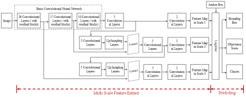
Our model consists of a feature extraction module and a object detection module. The latter is further split into bounding box detection and class detection. The overall architecture of the model is illustrated in Figure 1 below.
Figure 1. Architecture of the CSSS detection model
2.1 Feature extraction module
In the feature exaction module, all features are divided into three scales, and extracted from the corresponding FOV image based on a concept similar to the feature pyramid network [15]. To prevent the pooling-induced loss of low-level features, the module is entirely made up of convolutional layers, with no pooling layer. The stride of convolution kernels was set to 2 to ensure the down-sampling effect. Drawing on the structure of the ResNet, 3*3 and 1*1 kernels were arranged continuously in each convolutional layer, and supported with some interlayer connections.
Firstly, a basic CNN with 53 convolutional layers was constructed to extract the basic features. There are 23 residual blocks in the basic CNN. The structure of each block is the same as what is specified in Reference [12]. In this structure, a few shortcut connections are designed to avoid the vanishing gradient problem in network training. Thus, the network architecture becomes deeper and more capable of extracting image features. The structure of the basic CNN for feature extraction is described in Table 1 below.
Table 1. Structure of the basic CNN for feature extraction
|
Repetition |
Type of layer |
Number of filters |
Stride |
Filter Size |
Output |
|
|
Convolutional |
32 |
|
3 × 3 |
256×256 |
|
|
Convolutional |
64 |
2 |
3 × 3 |
128×128 |
|
1 × |
Convolutional |
32 |
|
1 × 1 |
|
|
Convolutional |
64 |
|
3 × 3 |
|
|
|
Residual |
|
|
|
128×128 |
|
|
|
Convolutional |
128 |
2 |
3 × 3 |
64×64 |
|
2 × |
Convolutional |
64 |
|
1 × 1 |
|
|
Convolutional |
128 |
|
3 × 3 |
|
|
|
Residual |
|
|
|
64×64 |
|
|
|
Convolutional |
256 |
2 |
3 × 3 |
32×32 |
|
8 × |
Convolutional |
128 |
|
1 × 1 |
|
|
Convolutional |
256 |
|
3 × 3 |
|
|
|
Residual |
|
|
|
32×32 |
|
|
|
Convolutional |
512 |
2 |
3 × 3 |
16×16 |
|
8 × |
Convolutional |
256 |
|
1 × 1 |
|
|
Convolutional |
512 |
|
3 × 3 |
|
|
|
Residual |
|
|
|
16×16 |
|
|
|
Convolutional |
1, 024 |
2 |
3 × 3 |
8×8 |
|
4 × |
Convolutional |
512 |
|
1 × 1 |
|
|
Convolutional |
1, 024 |
|
3 × 3 |
|
|
|
Residual |
|
|
|
8×8 |
|
|
|
Average Pooling |
|
|
Global |
|
|
|
Fully-connected |
|
|
1000 |
|
Next, several convolutional layers were added to extract features of different scales. The feature map was acquired from the shallow layers of the network, and then merged with the up-sampling function via connections. This allows us to obtain more fine-grained information of the previous feature map, while mining more meaningful semantic information from up-sampling features. The hybrid feature map of the two types of information was processed by the subsequent convolutional layers, laying the basis for predicting the detection results. The features of different scales are extracted in the following steps.
Firstly, the detected features of the first scale were obtained after the 79th layer. Compared to the input image, the feature map was down-sampled 32 times. If the size of the input image is 416×416, then the size of the feature map will be 13×13. Due to the high down-sampling factor, the feature map has a relatively large receptive field, which is suitable for detecting large objects in the image.
The second step is to obtain more fine-grained information. Up-sampling was conducted rightwards from the feature map of the 79th layer. The up-sampled result was concatenated with the feature map of the 61st layer, forming a fine-grained feature map of the 91st layer. Compared to the input image, the feature map was down-sampled 16 times through a few convolutional layers. The down-sampled feature map has a medium receptive field, and is suitable for detecting medium-sized objects.
Finally, the feature map of the 91st layer was up-sampled and then concatenated with the feature map of the 36th layer, forming a feature map down-sampled 8 times relative to the input image. This feature map has a small receptive field and is suitable for detecting small objects.
Based on each of the three feature maps, a three-dimensional (3D) tensor was predicted to encode the forecasts of bounding box, object and class.
2.2 Object detection module
The object position is not fixed in the FOV image or video, but constantly changing with the visual angle and position of the user. An object may appear anywhere in the FOV. Neither does the object have a fixed size in the FOV, for its distance to the observer varies with the latter’s position. Hence, the object detection algorithm should firstly find all the areas that may contain objects, treat them as anchor boxes, and identify and classify objects based on these anchor boxes.
In our model, the anchor boxes are identified by dimensional clustering [16]. The size of each anchor box needs to be adjusted according to the changing number and scale of output feature maps. In this paper, the k-means clustering is employed to produce anchor boxes of different sizes. Three anchor boxes were generated for each scale, and are suitable for detecting objects on the corresponding scale. The three large anchor boxes were applied to the large feature map (with a large receptive field), the three medium anchor boxes were applied to the medium feature map (with a medium receptive field), and the three small anchor boxes were applied to the small feature map (with a small receptive field).
Each FOV image was divided into S×S units, depending on the size of the feature map. If the center point of the object falls in one of the units, then this object will be detected by that unit. Each unit needs to predict three bounding boxes and their confidences. The confidence reflects the probability that a bounding box contains object(s). Here, it is defined as $\operatorname{Pr}(\text { Object }) * \text { IO } U_{\text {pred }}^{\text {truth}}$. If no object appears in the unit, then the confidence will be equal to zero; otherwise, the confidence is expected to be the intersection over union (IOU) between the predicted and ground-truth bounding boxes:
$I O U=\frac{P \cap G}{P \cup G}$
where, P is the bounding box predicted by the model; G is the ground-truth bounding box. Each bound box has five predicted values, namely, x, y, w, h and confidence. The (x, y) are the predicted coordinates of the bounding box relative to the unit; w and h are the predicted width and height relative to the entire image, respectively. For each bounding box, four coordinates were predicted by our model: tx, ty, tw and th. Let pw and ph be the width and height of the anchor box. If the bounding box stretches beyond the upper left corner (cx, cy) of the unit, then the final predicted coordinates of the bounding box can be expressed as:
$\begin{array}{c}{b_{x}=\sigma\left(t_{x}\right)+c_{x}} \\ {b_{y}=\sigma\left(t_{y}\right)+c_{y}} \\ {b_{w}=p_{w} e^{t_{w}}} \\ {b_{h}=p_{h} e^{t_{h}}}\end{array}$
During model training, the sum of squares for error (SSE) was taken as the loss function. Since the gradient of the model equals the ground-truth value t* minus the predicted value t*, the ground-truth value can be derived from the predicted value and the gradient. Our model predicts the confidence score of each bounding box through logistic regression. The score of a bounding box equals one, if the overlap between the a priori value of the box and the ground-truth value is greater than that of any other box. Inspired by Ren et al. [17], there is no need to predict this score, if the overlap is not optimal but greater than a threshold (0.5). In our model, each ground-truth value is assigned one bounding box only. If the previous bounding box has not been assigned to any ground-truth value, the prediction of coordinates or class will not be affected. The only thing being affected is the judgment of whether a bounding box contains objects.
Each unit also predicts C class conditional probabilities,$\operatorname{Pr}\left(\text {Class}_{i} | \text {Object}\right)$. These probabilities are the chances that the unit has only one object. The classes of the objects in each bounding box were predicted by multi-label classification. Different from the other CNNs, our CNN model replaces the softmax function in the output layer with independent logical classifiers. The class classifiers were trained with the loss function of binary cross-entropy. That is why our model performs well in the recognition of complex objects. For example, some datasets have many overlapping tags (e.g. women and human). This goes against the assumption of the softmax function that each bounding box has only one class. During testing, the class conditional probability of each bounding box was multiplied with the confidence of that box:
$\begin{aligned} \operatorname{Pr}(\text {Class_i } \text { Object }) & * \operatorname{Pr}(\text { Object }) * \text {IOU}_{\text {pred}}^{\text {truth}} \\ &=\operatorname{Pr}\left(\text {Class}_{i}\right) * \text {IOU}_{\text {pred}}^{\text {truth}} \end{aligned}$
This gives us the confidence score for each class in the bounding box. The score reflects how likely the class may appear in the bounding box and how suitable is the box size.
Through the above steps, our CNN output many detection boxes with confidence scores for different objects. The detection boxes may contain or overlap each other, and the contained objects may be the same or difference. In general, a high confidence means a good chance for the detection box to contain object(s). However, high confidence detection boxes may target the same object with obvious features. Thus, some objects may be overlooked if the top detection boxes are selected simply from the confidence ranking. To solve the problem, the detection boxes were screened by the non-maximum suppression (NMS) algorithm. The NMS is a local maximum search method. Here, “local” stands for a neighborhood containing two variables (i.e. the dimensions and size). The main idea of the NMS is to identify local maxima and suppress local minima according to certain comparison rules. Let S be the set of detection boxes with confidence scores and S′be the set of detection boxes after the screening. Then, the steps of the NMS are listed below.
Step 1. Sort the detection boxes in set S by confidence score.
Step 2. If the set S is not empty, perform the following:
(a) Select the detection box with the highest confidence score from the set S;
(b)Insert w into the set S’;
(c) Compare each of the remaining detection box in set S with w. If it overlaps w at a ratio greater than the threshold (e.g. 0.6), remove the box from the set S.
2.3 Comparative analysis
Our model was compared with a popular object detection method region-CNN (R-CNN) and its variants like Fast R-CNN [18]/Faster R-CNN [17]. The following similarities and differences were discovered through the comparison.
The R-CNN and its variants search for the objects in the image using the region proposal network (RPN) [19] rather than sliding windows [17]. To minimize duplicate detections, the potential bounding boxes are searched for selectively, the features are extracted with the CNN, the scores of bounding boxes are evaluated by the support vector machine (SVM) and the bounding boxes are adjusted by the linear model. In this complex process, each phase must be adjusted independently and accurately, which slows down the detection speed. It takes more than 40s for the R-CNN and its variants to detect the objects in each image. Thus, these methods cannot achieve the real-time performance of human eyes.
Our model has some similarities to the R-CNN. For example, the potential bounding boxes are proposed by each unit, and rated based on convolutional features. Nevertheless, our model sets a space limit on the unit proposals, such that the same object will not be detected multiple times. Another difference lies in the small number of bounding boxes in our model, which speeds up the detection process. In addition, our model is a universal detector that can detect multiple objects simultaneously and get close to the visual effects of human eyes. That is why our model outputs better analysis results than the contrastive models.
The convolutional layers of our model were pretrained on an ImageNet dataset containing 1, 000 classes of data [20]. In this process, the first 53 convolutional layers and the fully-connected layer in Figure 1 were trained to reach the top-5 accuracy of 88 % on ImageNet 2012 dataset, that is, the network has a comparable capacity to GoogLeNet. The research of Ren et al. shows that the network performance can be improved by adding convolutional layers and fully-connected layer to the pretrained network [21]. Therefore, it is enough to pretrain only the first 53 convolutional layers. After the pretraining, the above-mentioned CNN structures that extract features on three different scales were superimposed on the pretrained CNN, and then subjected to further training.
The last layer of the network is responsible for predicting the class probability and bounding box coordinates at the same time. Here, the width and height of each bounding box are normalized to the interval [0, 1] based on those of the image. In addition, a linear activation function was adopted for the last layer, and the following leaky rectified linear activation function was selected for all the other layers:
$\phi(x)=\left\{\begin{array}{c}{\mathrm{x}, \text { if } \mathrm{x}>0} \\ {0.1 \mathrm{x}, \text { otherwise }}\end{array}\right.$
For simplicity, the model was optimized based on the SSE of its outputs. However, this optimization approach is not the best choice to maximize the mean accuracy, as it assigns the same weight to the positioning error and classification error. Moreover, many units contain no object in each image. If the confidence of such a unit is simply set to zero, the gradient of the units containing object(s) will be suppressed. In this case, the model will behave unstably, and even fail to converge in the early phase of training. To solve this problem, the loss between the predicted and ground-truth coordinates of each bounding box was increased by a parameter λcoord(5) and the loss between the predicted and ground-truth confidences of each box containing no object was decreased by a parameter λcoord(0.5). In addition, the summation error can also increase the errors in large and small bounding boxes. To reflect the fact that a large bounding box has a lower small deviation than a small bounding box, this paper directly predicts the square root of the width and height of each bounding box, rather than the width and height.
In our model, each unit is responsible for the prediction of multiple bounding boxes. The training aims to ensure that each object is handled by one bounding box predictor. For an object, the predicted bounding box with the highest IOU was selected as the final bounding box to predict that object. Hence, the bounding box detection can make predictions of size, width-height ratio or class on different scales, thus increasing the overall recall rate.
During model training, the loss function was optimized as follows:
$\begin{align} & {{\lambda }_{\text{coord}}}\sum\limits_{i=0}^{{{S}^{2}}}{\sum\limits_{j=0}^{B}{\mathbb{I}_{i}^{\text{obj}}}}\left[ {{\left( {{x}_{i}}-{{{\hat{x}}}_{i}} \right)}^{2}}+{{\left( {{y}_{i}}-{{{\hat{y}}}_{i}} \right)}^{2}} \right] \\ & +{{\lambda }_{\text{coord}}}\sum\limits_{i=0}^{{{S}^{2}}}{\sum\limits_{j=0}^{B}{\mathbb{I}_{i}^{\text{obj}}}}\left[ {{(\sqrt{{{w}_{i}}}-\sqrt{{{{\hat{w}}}_{i}}})}^{2}} \right.\left. +{{(\sqrt{{{h}_{i}}}-\sqrt{{{{\hat{h}}}_{i}}})}^{2}} \right] \\ & +\sum\limits_{i=0}^{{{S}^{2}}}{\sum\limits_{j=0}^{B}{\mathbb{I}_{i}^{\text{obj}}}}{{(\sqrt{{{C}_{i}}}-\sqrt{{{{\hat{C}}}_{i}}})}^{2}} \\ & +\cdot {{\lambda }_{\text{noobj}}}\sum\limits_{i=0}^{{{S}^{2}}}{\sum\limits_{j=0}^{B}{\mathbb{I}_{i}^{\text{obj}}}}{{(\sqrt{{{C}_{i}}}-\sqrt{{{{\hat{C}}}_{i}}})}^{2}} \\ & +\sum\limits_{i=0}^{{{S}^{2}}}{\mathbb{I}_{i}^{\text{obj}}}\sum\limits_{\text{c}\in \text{classes}}{{{\left( {{p}_{i}}(c)-{{{\hat{p}}}_{i}}(c) \right)}^{2}}} \\\end{align}$.
where $\prod_{i}^{O b j}$ indicates whether any object appear in unit i; $\prod_{i}^{O b j}$ means the bounding box predictor j of unit i is responsible for the prediction. Note that if the unit contains object(s), the loss function only penalizes the classification error (that is why the class conditional probabilities were discussed); if the predictor is “responsible” for the ground-truth bounding box (i.e. the unit contains the highest IOU), the loss function only penalizes the error in the bounding box coordinates.
4.1 Datasets
(1) Design and construction of scene models for the CSSS
There are mainly four types of VR technologies, namely, immersive VR, augmented reality (AR), desktop VR and distributed VR. The desktop VR was selected to generate the video of the observations of a user walking through the commercial space, laying the basis for computer analysis of dynamic images.
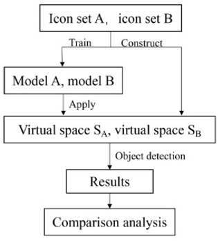
After surveying and summing up the common commercial spaces in China, the author designed and constructed a commercial building model with the features of modern commercial space. Then, the commercial signs containing effective information were placed into the model at proper intervals according to the function and business divisions. Thus, the entire CSSS belongs to the same space, i.e. the interior space (S) of the commercial building model. To compare the detectability difference of CSSSs of varied styles, two sets of signs (A and B) were designed and arranged in the same places within S, creating two virtual spaces (SA and SB). The two virtual spaces have the same spatial pattern and only differ in the sign style.
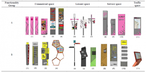
Considering the commercial behavior of the user, the large CSSS needs to familiarize the user with several kinds of spaces, including commercial space, leisure space, service space and traffic space. Besides, the large CSSS mainly expresses the following visual elements: form, graphic, color, material and word. The five elements were combined in different forms to achieve various visual effects, inducing different psychological and behavioral features of the user. The types and elements of the CSSS are presented in Figure 2.
Figure 2. Types and elements of the CSSS
The two CSSSs differ in each of the five elements. The first CSSS mainly uses graphics and exciting pinky colors, plus the dark grey color. By contrast, the second CSSS mainly uses words and adopts bright yellow and other bright colors. The two CSSSs are displayed by functionality group in Table 2.
Table 2. The two CSSSs
(2) Generation of VR videos
The VR models were generated by the virtual simulation software MARS. Specifically, an architectural model was established in the SKP format in the Sketchup software, and then imported to the MARS. To approximate the actual texture, the materials were selected from the material library of the software and placed on the corresponding places on the surface of the model. After that, the illumination and weather throughout the day were simulated by configuring the weather system and the time control module in the MARS, making the model more realistic. In the fully rendered model, the specific scenes of the space were set sequentially, and the time for video generation was also selected, making it possible to output coherence videos on different scenes. Finally, user walkthrough was conducted in SA and SB along the same route at the same speed, creating the video data in the walkthrough FOV of the two CSSSs.
4.2 Experimental procedure
The acquired walkthrough videos of the two CSSSs were analyzed with our model, yielding close-to-reality visual feedbacks. Then, the feedback data of the two CSSSs were compared in details. The specific flow is explained in Figure 3 below.
Figure 3. The object detection process of the two CSSSs
(1) Model training
The original design drawings of each CSSS were taken as the training set. Each set contains the signs in all 11 classes of each design plan. For each sign, there are eight images from different angles, i.e. the front, the rear, the two sides, and the four diagonal directions. In total, the training set has 96 images. Then, the training data were expanded by data enhancement. The original images were randomly scaled by 20 % and flipped. Besides, the exposure and saturation of the images were randomly increased to 1.5 times in the HSV color space.
The ResNet-based CSSS detection model was applied to extract feature maps of three scales, (13×13), (26×26) and (52×52), for each image in the training set. Then, three bounding boxes were predicted for each scale. Thus, a tensor of the size N×N×[3× (4+1+12)] was obtained to describe the predicted results, where N is the size of the scale (i.e. 13, 26 or 52). Each bounding box was coded in 17 digits, in which the first 4 digits are the coordinates of the box, the fifth is the object confidence and the last twelve are the predicted scores of each class.
On the setting of anchor boxes, 9 cluster heads and 3 scales were selected, and the anchor boxes were determined through k-means clustering of the training set. The obtained anchor boxes fall onto 9 scales: (10×13), (16×30), (33×23), (30×61), (62×45), (59×119), (116×90), (156×198) and (373×326). Next, the cluster heads were divided evenly on scale. On small13×13 feature maps (with a large receptive field), the large a priori boxes (116×90), (156×198) and (373×326) were applied to detect large objects; on medium 26×26 feature maps (with a medium receptive field), the medium a priori boxes (30×61), (62×45) and (59×119) were applied to detect medium objects; on large 52×52 feature maps, the small a priori boxes (10×13), (16×30) and (33×23) were applied to detect small objects.
The model was trained in batches of 64 images with a momentum term of 0.9, and an attenuation term of 0.0005. During the batch training, the learning rate was adjusted by the following strategy: In the early phase, the learning rate was slowly increased from 10-3 to 10-2, because the model may diverge due to gradient instability under a high initial learning rate; Then, the model was trained for 75 periods at the learning rate of 10-2, 30 iterations at 10-3 and finally 30 iterations at 10-4. To prevent over-fitting, the dropout layer and data expansion were introduced. Specifically, a dropout layer (dropout rate: 0.5) was added after the first fully-connected layer to eliminate the coadaptation between the layers [22].
Through the above training, two models were obtained for CSSS evaluation.
Table 3. Anchor box assignment for different scales
|
Feature map size |
13×13 |
26×26 |
52×52 |
||||||
|
Receptive field |
Large |
Medium |
Small |
||||||
|
Anchor box size |
116×90 |
156×198 |
373×326 |
30×61 |
62×45 |
59×119 |
10×13 |
16×30 |
33×23 |
(2) Interactivity analysis
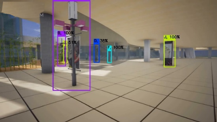
The obtained evaluation models were adopted to detect each frame of video sets SA and SB. The detection results include the position, class and confidence of each sign. Figure 4 presents the detection results of one frame in a VR walkthrough video.
Figure 4. The detection results of one frame in a VR walkthrough video
The design effects of the two CSSSs were compared by analyzing the detection results of each frame in the videos captured from the user’s visual angle. The confidence score is the most important indicator of the significance of a sign, i.e. whether the sign is easy to recognize and detect. In this experiment, the statistical analysis is employed to evaluate the sign significance, focusing on the mean and standard deviation of signs in each class. This is because the two videos were generated in the same visual angle and walking path. In addition, the confidence of the same sign increases gradually from a low level to 100 %, when the user walks towards the sign. The speed of this process (the mean detection time) is another indicator of the significance of the sign.
Meanwhile, the sign discrimination was evaluated by the false detection rate and the time to correct the false detection (the correction time). The false detection rate was not computed based on tags, due to the heavy workload and unnecessity of tagging each frame. Since any sign close enough to the observer can be recognized at 100 % confidence, the following strategy was proposed to evaluate sign discrimination, coupling the analysis of adjacent frames: With the increase of confidence for the same sign, any change in the recognized class means the sign has been falsely detected in the early phase, and the time before the change is the time to correct the false detection. The shorter the correction time, the higher the sign discrimination, and the better the visual experience of the user.
The experimental results of the two CSSSs are listed in Table 4.
Table 4. Statistical results of the two CSSSs
|
Property |
Index |
CSSS A |
CSSS B |
|
Significance |
Global mean confidence |
95.58 % |
97.52 % |
|
Global standard deviation of confidence |
0.0229 |
0.0134 |
|
|
Global mean detection time |
0.68s |
0.46s |
|
|
Discrimination |
Global false detection rate |
5.57 % |
1.07 % |
|
Global correction time |
0.28s |
0.11s |
In terms of significance, CSSS B had a smaller mean confidence and shorter mean detection time than CSSS A. This means the former can be recognized more easily by the user, and convey information to the user in the commercial building. The result agrees with the intuitive feeling that the brighter and more irregular signs in CSSS B are more eye-catching than those in CSSS A.
Figure 5. Mean confidences of signs in 11 classes in the two CSSSs
The mean confidence of the signs in each class of the two CSSSs is shown in Figure 5. It can be seen that the confidence of CSSS B was higher than that of CSSS A, and more stable from class to class (a smaller global standard deviation of confidence). The results show that the individual signs in CSSS B are closer in significance and more stable in visual effect than those in CSSS A.
In terms of discrimination, CSSS B had a much lower false detection rate and a shorter correction time than CSSS A, indicating that the signs of different classes in CSSS B are easier to differentiate than those in CSSS A. The high discrimination design makes it easier for the user to find a specific sign, and enhances the significance of signs. The results also agree well with the intuitive feeling that that the brighter and more irregular signs in CSSS B are easier to distinguish than those in CSSS A.
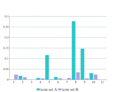
Figure 6. False detection rates of signs in 11 classes in the two CSSSs
The false detection rate of the signs in each class of the two CSSSs is shown in Figure 6. It can be seen that CSSS A had a higher false detection rate than CSSS B, especially in class 8 and class 9. From the angle of sign design, the high false detection rates of the two classes may be resulted from the similarity between them in appearance. Therefore, it is easy for the user to confuse between the signs in the two classes if he/she is far away. The two classes should be improved in the subsequent design.
To sum up, CSSS B outshines CSSS A in both significance and discrimination.
This paper puts forward a method to analyze and evaluate the interactive design of the CSSS based on object detection, aiming to effectively quantify the signs before use. Firstly, a virtual commercial building model was set up to mimic the walkthrough of the user in commercial space. Next, an object detection model was constructed based on the ResNet, which is an effective structure in computer vision. The model was adopted to simulate the visual experience of the user walking through the commercial space, and generate quantifiable experience data to analyze and evaluate the CSSS in the design phase. In addition, the quantification indices were put forward to evaluate the significance and discrimination of the signs. The experimental results show that these quantification indices are in line with the actual experience of human visual senses. This research provides a new quantitative analysis method for the evaluation of the CSSS design, shedding new light on design optimization in future research.
[1] Burnaz, S., Topcu, Y.I. (2011). A decision support on planning retail tenant mix in shopping malls. Procedia - Social and Behavioral Sciences, 24: 317-324. https://doi.org/10.1016/j.sbspro.2011.09.124
[2] Butler, D.L., Acquino, A.L., Hissong, A.A., Scott, P.A. (1993). Wayfinding by newcomers in a complex building. Human Factors the Journal of the Human Factors and Ergonomics Society, 35(1): 159-173. https://doi.org/10.1177/001872089303500109
[3] Li, H., Thrash, T., Hölscher, C., Schinazi, V. (2019). The effect of crowdedness on human wayfinding and locomotion in a multi-level virtual shopping mall. Journal of Environmental Psychology, 65: 101320 https://doi.org/10.1016/j.jenvp.2019.101320
[4] Motamedi, A., Wang, Z., Yabuki, N., Fukuda, T., Michikawa, T. (2017). Signage visibility analysis and optimization system using BIM-enabled virtual reality (VR) environments. Advanced Engineering Informatics, 32: 248-262. https://doi.org/10.1016/j.aei.2017.03.005
[5] He, K., Zhang, X., Ren, S., Sun, J. (2014). Spatial pyramid pooling in deep convolutional networks for visual recognition. IEEE Transactions on Pattern Analysis and Machine Intelligence, 37(9): 1904-1916. https://doi.org/10.1109/TPAMI.2015.2389824
[6] Szegedy, C., Toshev, A., Erhan, D. (2013). Deep neural networks for object detection. Advances in Neural Information Processing Systems, 2553-2561.
[7] He, K., Gkioxari, G., Dollari, P., Girshick. R. (2017). Mask R-CNN. IEEE Transactions on Pattern Analysis and Machine Intelligence (Early Access), 1-1. https://doi.org/10.1109/TPAMI.2018.2844175
[8] Jeon, Y., Kim, J. (2017). Active convolution: Learning the shape of convolution for image classication. 2017 IEEE Conference on Computer Vision and Pattern Recognition (CVPR). https://doi.org/10.1109/CVPR.2017.200
[9] Jarrett, K., Kavukcuoglu, K., Ranzato, M., LeCun, Y. (2009). What is the best multi-stage architecture for object recognition? 2009 IEEE 12th International Conference on Computer Vision. https://doi.org/10.1109/ICCV.2009.5459469
[10] Felleman, D.J., van Essen, D.C. (1991). Distributed hierarchical processing in the primate cerebral cortex. Cerebral Cortex, 1(1): 1–47. https://doi.org/10.1093/cercor/1.1.1
[11] Cadieu, C. F., Hong, H., Yamins, D.L., Pinto, N., Ardila, D Solomon, E.A., Majaj, N.J., DiCarlo, J.J. (2014). Deep neural networks rival the representation of primate it cortex for core visual object recognition. PLoS Computational Biology, 10(12): e1003963. https://doi.org/10.1371/journal.pcbi.1003963
[12] He, K.M., Zhang, X.Y., Ren, S.Q., Sun, J. (2015). Deep residual learning for image recognition. arXiv preprint arXiv: 1512.03385. https://doi.org/10.1109/CVPR.2016.90
[13] Greff, K., Srivastava, R.K., Koutník, J., Steunebrink, B.R., Schmidhuber, J. (2016). LSTM: A search space odyssey. IEEE Transactions on Neural Networks and Learning Systems, 28(10): 2222-2232. https://doi.org/10.1109/TNNLS.2016.2582924
[14] Donahue, J., Hendricks, L.A., Rohrbach, M., Venugopalan, S., Guadarrama, S., Saenko, K., Darrell, T. (2017). Long-term recurrent convolutional networks for visual recognition and description. IEEE Transactions on Pattern Analysis and Machine Intelligence, 39(4): 677-691. https://doi.org/10.1109/TPAMI.2016.2599174
[15] Lin, T.Y., Dollar, P., Girshick, R., He, K., Hariharan, B., Belongie, S. (2017). Feature pyramid networks for object detection. 2017 IEEE Conference on Computer Vision and Pattern Recognition, 2117–2125. https://doi.org/10.1109/CVPR.2017.106
[16] Redmon, J., Farhadi, A. (2017). Yolo9000: Better, faster, stronger. 2017 IEEE Conference on Computer Vision and Pattern Recognition (CVPR), 6517–6525. https://doi.org/10.1109/CVPR.2017.690
[17] Ren, S., He, K., Girshick, R., Sun, J. (2015). Faster R-CNN: Towards real-time object detection with region proposal networks. Advances in Neural Information Processing Systems, 91-99. https://doi.org/10.1109/TPAMI.2016.2577031
[18] Girshick, R.B., (2015). Fast R-CNN. 2015 IEEE International Conference on Computer Vision (ICCV). https://doi.org/10.1109/ICCV.2015.169
[19] Uijlings, J.R., van de Sande, K.E., Gevers, T., Smeulders, A.W. (2013). Selective search for object recognition. International Journal of Computer Vision IJCV, 104(2): 154-171. https://doi.org/10.1007/s11263-013-0620-5
[20] Russakovsky, O., Deng, J., Su, H., Krause, J., Satheesh, S., Ma, S., Huang, Z., Karpathy, A., Khosla, A., Bernstein, M., Berg, A.C., Li, F.F. (2015). ImageNet large scale visual recognition challenge. International Journal of Computer Vision (IJCV), 115(3): 211-252. https://doi.org/10.1007/s11263-015-0816-y
[21] Ren, S., He, K., Girshick, R., Zhang, X., Sun, J. (2015). Object detection networks on convolutional feature maps. IEEE Transactions on Pattern Analysis and Machine Intelligence, 39(7): 1476-1481. https://doi.org/10.1109/TPAMI.2016.2601099
[22] Hinton, G.E., Srivastava, N., Krizhevsky, A., Sutskever, I., Salakhutdinov, R.R. (2012). Improving neural networks by preventing co-adaptation of feature detectors. arXiv preprint arXiv:1207.0580.