Hong Zhou* | Kunming Yu
OPEN ACCESS
Data aggregation is an efficient method to save energy and prolong the service life of wireless sensor networks (WSNs). In light of this, a data aggregation algorithm was constructed based on self-organizing feature mapping (SOFM) neural network and WSN cluster routing protocol. In this algorithm, each cluster was designed as a three-layer neural network model, which collect a large number of raw data. Then, the feature data were extracted from the raw data, and sent to the sink node. Through a simulation experiment, it is proved that the proposed algorithm, denoted as SOFMDA, outperformed a popular data aggregation method in energy consumption and data accuracy.
wireless sensor networks (WSNs), self-organizing feature mapping (SOFM), neural network, data aggregation, feature extraction
Wireless sensor networks (WSNs) has been applied into Industry 4.0 for monitoring the production environment and the production process. In a typical industrial WSN, multiple sensor nodes are often deployed in a specific area to realize full coverage with some overlapping sensing ranges. Due to the high spatial correlation of the sensing area, the data collected by these nodes are very similar, most of which are redundant and will cause a large amount of resources waste to store, transfer, process and calculate them. Furthermore, the more redundant sensing data needs the bigger storage space, the more transmission energy, the more complex data analysis and so on.
In view of the above, this paper puts forward a WSN data aggregation algorithm based on self-organizing feature mapping (SOFM) neural network, denoted as SOFMDA. Considering the location-based clustering routing protocol in the WSN, this method utilizes the SOFM neural network to analyze and classify the sensing data and extract data features in order to deduce the redundant data and then make a reduction of the storage space, the transmission load and energy consumption and simplify the continued data mining process.
2.1 SOFM neural network
Self-Organizing Feature Map (SOFM) is a mathematical models for information processing of structures similar to the self-organizing characteristics of human brain. It adopts unsupervised learning rules for network training, which is different from the Artificial neural networks (ANNs) applied supervised learning rules [1].
SOFM network has two layers. The input layer neurons aggregate the external information to the output layer neurons through the weight vector. The number of neurons in the input layer is equal to the sample dimension.
The arrangement of neurons has many forms, such as one-dimensional linear array, two-dimensional planar array and three-dimensional grid array. One-dimensional and two-dimensional arrays are common. One-dimensional structure is the simplest. The structural characteristics are shown in Figure 1. There are lateral connections between neurons in each competitive layer.
Figure 1. Structure of one-dimensional SOFM network
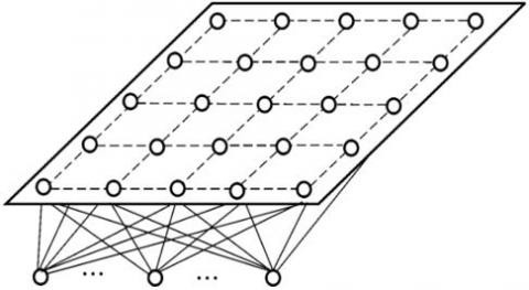
Output is the most typical organization of SOFM network in two-dimensional plane. Each neuron in the output layer is connected laterally with other neurons around it and arranged in a chessboard plane. Its structure is shown in Figure 2.
Figure 2. Structure of two-dimensional SOFM network
The training process of SOFM neural network is:
Step1: a small random initial value is preset for the reference vector of all output neurons.
Step2: provide a training input mode for the network.
Step3: determine the winning output neuron, that is, the neuron whose reference vector is closest to the input mode. The Euclidean distance between the reference vector and the input vector is usually used as a distance measurement.
Step4: update the reference vector of the winning neuron and its neighbors according to the Kohoen’s learning rule. The weight vector of each winning neuron lies closest to the input vector, and all the neurons in its neighborhood are subjected to weight update.For example, the weights of a winning neuron (nodei) and the nodes in its neighborhood If the ith neuron in the competition layer wins, its weight vector wi will be modified as:
$w i(k)=w i(k-1)-\alpha(P(k)-w i(k-1))$ (1)
where, w is marked as weight; k is the number of training rounds; $\alpha$ is the learning rate correlated to the learning effect and computing load. If $\alpha$ is too large, the learning results may be poor due to insufficient training; if $\alpha$ is too small, the network may not be able to achieve the learning goals in the long run.
2.2 Data aggregation methods
Heidari et al. [2] put forward a WSN data aggregation algorithm to overcome the defects of the low energy adaptive clustering hierarchy (LEACH) algorithm in cluster head selection, data aggregation and routing between cluster head and the base station, and verified the improvement effect through simulation experiments. In the WSN data aggregation algorithm, energy control conditions are added to the cluster head selection, and the routing between cluster head and the base station is replaced with a multi-hop reverse multicast tree suitable for data aggregation.
Based on spatial correlations, Wang et al. [3] developed a data aggregation algorithm that classifies and fuses sensor data according to the spatial location and data features, and proved that the algorithm outperforms the reliability assessment algorithm (RAA) in energy consumption, data acquisition and aggregation effect.
Akkaya et al. [4] presented a data-centric aggregation technique, i.e. a fuzzy clustering (VF) algorithm, based on Voronoi diagram, and confirmed through simulation experiments that the algorithm can effectively improves the network performance. In this algorithm, the data are aggregated at the cluster head, in light of the residual nodal energy, the service quality and the distance between the cluster head and the neighbor node.
2.3 Application of neural networks in WSNs
Much research has been done on the application of neural networks in WSNs. For instance, Sharaf et al. [5] uses multi-layer perceptron (MLP) neural networks to identify abnormal events based on the WSN signal changes. Attea and Khalil [6] created an adaptive routing algorithm for the WSN based on neural network, and verified through simulation experiments that the algorithm is 0.8 times more efficient than the efficient multi-hop hierarchical routing (EMHR) algorithm; in this algorithm, the cluster head is selected through neural network adaptive learning at the base station and the next hop in the shortest path is determined according to the optimal weight function.
Barbancho et al. [7] applied SOFM neural network to the WSN for the first time, and proposed a wireless sensor routing protocol based on the SOFM, which fails to consider data aggregation. Sung [8] completed data aggregation using a three-layer perceptron neural network, which is developed from backpropagation (BP) neural network and WSN clustering routing protocol, and discovered that the neural network can outshine the LEACH algorithm if there is a training output set [9]. Inspired by Sung, Zhang et al. [10] introduced the processing of data features to the LEACH algorithm and found that the improved algorithm cannot work without training output set.
None of the existing methods can effectively achieve good results through neural network training. Considering the above, this paper introduces the SOFM neural network to the WSN for data aggregation, taking the WSN nodes as neurons in the neural network and the collected data as the neuron inputs. The incremental learning of the neural network was performed in the cluster head before data classification. Such a neural network with unsupervised learning rules was adopted because it is impossible to know the correct classification of training data in advance.
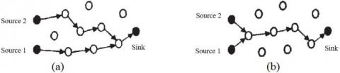
The selection of data aggregation points is a very important and key problem in SOFMDA algorithm. The effect of data aggregation points on data aggregation is compared through two simple examples in Figure 3. The data aggregation point in Figure 3 (a) is closer to the sink node, while the data aggregation point in Figure 3 (b) is closer to the data source.
Figure 3. The effect of data aggregation points on data aggregation
Obviously, the closer the data aggregation point is to the data source, the better the effect of data aggregation.
At the same time, the choice of data aggregation point mainly depends on the design of routing protocol. Especially in clustering routing protocols, cluster head nodes are ideal data aggregation points, because all cluster members send the collected data to their corresponding cluster head nodes. The location of cluster members is relatively close, and the data redundancy is relatively high. It is one of the main theoretical foundations of the SOFMDA data aggregation model in this paper.
3.1 SOFMDA model
Figure 4 shows a schematic diagram of the SOFMDA model, which uses a three-layer sensor neural network model that corresponds to a cluster in a WSN. The input layer and the first hidden layer are located in the cluster member node, and the output layer and the second hidden layer are located in the cluster head node.
Figure 4. Structure of SOFMDA aggregation model
There are n cluster member nodes in a cluster of WSN and each of them collects m different types of data. The neural network model has $n \times m$ input layer nodes and $n \times m$ first hidden layers neurons. The number of second hidden layer neurons s and the number of output layer neurons k can be adjusted according to the actual application needs, and they are not necessarily related to n. The number of second hidden layers may be different for different types of data. No full connection is used between the input layer and the first hidden layer, and between the first hidden layer and the second hidden layer, but different types of data are processed separately; and the second hidden layer and the output layer are fully connected, different types of data can be processed.
According to such a three-layer sensor neural network model, the SOFMDA data aggregation algorithm first performs initial processing on all collected data using the first hidden layer neuron function. Then send the processing result to the cluster head node of its cluster. The cluster head node further processes the data using the second hidden layer neuron function and the output layer neuron function. Finally, the cluster head node sends the processing result to the sink node.
In different wireless sensor network applications, according to the specific requirements of the application, the neural network model of the SOFMDA algorithm can be adjusted. In applications where data processing is relatively simple, the second hidden layer in the cluster head node can be combined with the output layer. In some applications where data processing is particularly complex, one or more hidden layers can be added to form a more complex neural network.
From the point of view of the overall wireless sensor network, one sensor node is considered as one of the bottommost neurons. The cluster head node is an intermediate neuron that acts as a convergence, and the entire network can be seen as a complex nervous system.
3.2 Neural model of SOFMDA
The artificial neuron model, the connection of artificial neurons, and the training and learning of artificial neural networks are the three key elements in the study of a specific neural network. The structure of the SOFMDA model mainly solves the connection of neurons. The neuron model of the SOFMDA will be discussed below.
Neurons are information processing units in neural networks. Neuron models are used to define the specific functions of neurons and how neurons process information. In general, neuron models are used to define the process of data aggregation.
In the SOFMDA data aggregation algorithm, the first hidden layer neuron is located at a cluster member node. The number of first hidden layer neurons is determined based on the type of data collected by the sensor nodes. Assuming that the number of types of data collected by the sensor node is n, then there are n single input first hidden layer neurons in each sensor node. In other words, different types of data are processed by different neuron
The input area function uses a weighted sum method. However, since each first hidden neuron has only one input signal, the input area function actually becomes an identity function. In other words, the result of the operation in the input area is the input signal itself.
The two functions of the processing area first calculate the absolute value of the difference between the current input data and the last recorded data, and then determine and decide whether to record the current input data.
The function of the output area uses a special threshold function: when $a_{1}(t)$ is less than the threshold $\theta_{1}$, the neuron has no output result; when $a_{1}(t) \geq \theta_{1}$, the output of the neuron is $a_{2}(t)$.
The second hidden layer neuron is located in the cluster head node of the wireless sensor network. The hierarchical neuron function is closely related to the specific application. The number of neurons in the second hidden layer and the functional function of each second hidden layer neuron depend on the specific application. Even the number of layers in the hidden layer of the cluster head node varies with the application requirements.
Similar to the first hidden layer neuron model, the second hidden layer neuron model of the SOFMDA is also composed of the input area function, the processing area function, and the output area function.
Similar to the second hidden layer neuron, the output layer neurons are also located in the cluster head node of the wireless sensor network, and the number of output layer neurons can also be determined according to the specific requirements of the application.
In the SOFMDA data aggregation algorithm, the design of the output layer neuron model is very similar to that of the first hidden layer neuron model. The biggest difference between them is that the first hidden layer neuron is single input neuron, and the output layer neuron is multiple input neuron. Figure4 shows an output layer neuron model of the SOFMDA.
In the input region of the output layer neuron, weighted sum functions are used, and the input data is the output of the second hidden layer. Similar to the first hidden layer neuron, the output layer neuron determines whether the difference between the latest results of weighted sum and the previous results of weighted sum exceeds the threshold $\theta_{2}$. If the difference exceeds the threshold $\theta_{2}$, the output of the neuron is the latest weighted sum. The cluster head node will send the latest weighted sum to the sink node.
The weight $w_{1}, w_{2}, \dots w_{n}$ is crucial for the output layer neurons. It is an important parameter of the SOFMDA model. In some neural networks, these weights can be learned, trained, and adjusted through the network itself. In the wireless sensor network, due to the limitations of system resources such as communication, CPU and storage space, it is impossible to train the weights within the wireless sensor network. Therefore, the SOFMDA model does not train these weights, but does this outside the wireless sensor network. Then, the weight parameter can be sent to all sensor nodes through the aggregation node. In practical applications, the weight changes very slowly, and the sink node does not send these parameters to the sensor nodes frequently.
SOFMDA data aggregation model is simulated. Each sensor node continuously collected the ambient temperature and relative humidity. After the SOFMDA aggregation processing, the cluster head node sent the temperature and humidity comprehensive index to the sink node.
In the test, the SOFMDA model was evaluated mainly through two indicators: (1) Average energy consumption of sensor nodes. It only calculates the energy consumed by the wireless transceiver module to send and receive messages. It does not include other hardware modules (such as MCUs and sensors). (2) Average communication load: It calculates the number of times the sensor node needs to send a data packet to the sink node (the average number of hops from the data source node to the sink node).
In order to test the performance of SOFMDA under different network sizes, six different scale WSN scenarios were selected: 75, 108, 147, 192, 243, and 300 sensor nodes were distributed at 600×500 m2, 720×600 m2, 840×700 m2, 960 × 800 m2, 1080 × 900 m2, and 1200 × 1000 m2 respectively. They have the same node density and good comparability. There is only one aggregation node in each network scenario, which is located in the center of the network.
In the SOFMDA, the threshold $\theta_{1}$ of the first hidden layer and the threshold $\theta_{2}$ of the output hidden layer are both 0.2. In the routing protocol, the grid width is fixed at 200m and the cluster head grid election period is 20s.
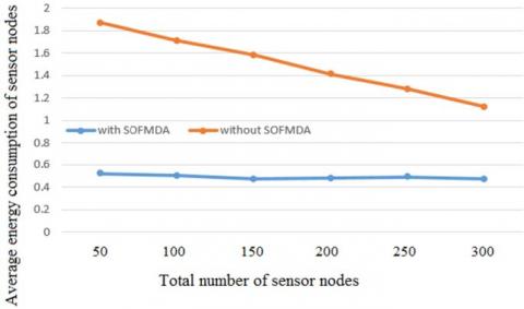
Figure 5 shows the comparison of the average energy consumption of sensor nodes using the SOFMDA data aggregation algorithm under different network sizes.
Figure 5. Effect of SOFMDA aggregation model on average energy consumption of nodes
Through the analysis of the results, the following conclusions can be drawn: (1) The average energy consumption of sensor nodes using SOFMDA data aggregation algorithm is lower than that when they are not used; (2) Regardless of whether or not the SOFMDA algorithm is used, as the network size increases (the number of sensor nodes increases), the average power consumption of the sensor nodes always decreases, but the decline rate is larger when the SOFMDA algorithm is not used.
Figure 6 shows the average traffic load comparison results using the SOFMDA data aggregation algorithm for different network sizes. Through the analysis of the results, the following conclusions can be drawn: (1) The average communication load of sensor nodes using SOFMDA data aggregation algorithm is lower than that when they are not used (2) Without the use of the SOFMDA algorithm, as the network scale increases (the number of sensor nodes increases), the average traffic load increases significantly, with a minimum value of 3.72 and a maximum value of 5.28. (3) With the increase in the size of the network (increase in the number of sensor nodes), the average communication load did not increase significantly, with a minimum value of 0.82 and a maximum value of 1.02.
Figure 6. The effect of SOFMDA aggregation model on average communication load
From the result of the simulation test, after using the SOFMDA data aggregation algorithm, it effectively reduced the communication load in the network and played a role in saving energy consumption.
In order to test the effect of the threshold value $\theta_{1}$ of the first hidden layer and the threshold $\theta_{2}$ of the output hidden layer on the performance of SOFMDA, three wireless sensor network topology structures are randomly selected. Each topology is randomly distributed in a region of 1200×1000 m2 size by 300 sensor nodes, and the converging node is located in the middle of the network. In SOFMDA, the threshold value $\theta_{1}$ of the first hidden layer and the threshold $\theta_{2}$ of the output hidden layer choose 0, 0.05, 0.1, 0.15, 0.2, 0.25 and 0.3, respectively. In the GROUP protocol, the grid width is fixed to 200m, and the cluster head grid election period is 20s.
Although the simulation test results show that the larger the first hidden layer threshold $\theta_{1}$ and the output hidden layer threshold $\theta_{2}$, the better data aggregation efficiency can be obtained. And it will have a negative impact on the authenticity and effectiveness of the data aggregation results. In addition, the simulation test results also show that too large $\theta_{1}$ and $\theta_{2}$ have little significance for data aggregation efficiency. Therefore, in practical applications, the values of the first hidden layer threshold $\theta_{1}$ and the output hidden layer threshold $\theta_{2}$ should take into account the efficiency of data aggregation and the effectiveness of the data.
his paper proposes a WSN data aggregation algorithm based on SOFM neural network, and denotes it as the SOFMDA. Considering the location-based clustering routing protocol in the WSN, the intra-cluster nodes were taken as the input layer neurons of the SOFM neural network, while the cluster head nodes, relying on the SOFM neural network, classify the data and extract data features, and then send the feature data to the sink node, thereby reducing the transmission load and energy consumption. Through a simulation experiment, it is proved that the proposed SOFMDA can effectively reduce the transmission volume through the classification of original data and the extraction of similar data features. The research findings shed new light on energy reduction, channel pressure relief, channel utilization improvement and service life extension of WSNs.
[1] Heidemann J, Silva F, Intanagonwiwat C, Govindan R, Estrin D, Ganesan D. (2001). Building efficient wireless sensor networks with low-level naming. Acm Sigops Operating Systems Review 35(5): 146-159. https://doi.org/10.1145/502034.502049
[2] Heidari E, Movaghar A, Mahramian M. (2010). The usage of genetic algorithm in clustering and routing in wireless sensor networks. Advances in Intelligent & Soft Computing 67: 95-103. https://doi.org/10.1007/978-3-642-10687-3_9
[3] Wang YH, Lin YW, Lin YY, Chang HM. (2013). A grid-based clustering routing protocol for wireless sensor networks. Advances in Intelligent Systems and Applications 1: 491-499. https://doi.org/10.1007/978-3-642-35452-6_50
[4] Akkaya K, Demirbas M, Aygun RS. (2010). The impact of data aggregation on the performance of wireless sensor networks. Wireless Communications & Mobile Computing 8(2): 171-193. https://doi.org/10.1002/wcm.454
[5] Sharaf MA, Beaver J, Labrinidis A, Chrysanthis PK. (2004). Balancing energy efficiency and quality of aggregate data in sensor networks. Vldb Journal 13(4): 384-403. https://doi.org/10.1007/s00778-004-0138-0
[6] Attea BA, Khalil EA. (2012). A new evolutionary based routing protocol for clustered heterogeneous wireless sensor networks. Applied Soft Computing Journal 12(7): 1950-1957. https://doi.org/10.1016/j.asoc.2011.04.007
[7] Barbancho J, León C, Molina FJ, Barbancho A. (2007). Using artificial intelligence in routing schemes for wireless networks. Computer Communications 30(14): 2802-2811. https://doi.org/10.1016/j.comcom.2007.05.023
[8] Sung WT. (2010). Multi-sensors data fusion system for wireless sensors networks of factory monitoring via BPN technology. Expert Systems with Applications 37(3): 2124-2131. https://doi.org/10.1016/j.eswa.2009.07.062
[9] Guhaneogi SA, Bhaskar A, Chakrabarti P. (2014). Energy efficient hierarchy-based clustering routing protocol for wireless sensor networks. International Journal of Computer Applications 95(13): 1-8. https://doi.org/10.5120/16651-6627
[10] Zhang SK, Cui Z.M, Gong SR, Sun Y, Fang W. (2009). A data fusion algorithm based on bayes sequential estimation for wireless sensor network. Journal of Electronics & Information Technology 31(3): 716-721. https://doi.org/10.1360/972009-1549
[11] Cai ZY, Liu CM, Liu Y, Ye QD. (2013). Application of high performance data fusion algorithm in wireless sensor network. Journal of Qingdao University of Science and Technology (Natural Science Edition) 34(3): 309-314. https://doi.org/10.3969/j.issn.1672-6987.2013.03.019
[12] Heinzelman WB, Chandrakasan AP, Balakrishnan H. (2002). An application-specific protocol architecture for wireless microsensor networks. IEEE Trans Wireless Commun 1(4): 660-670. https://doi.org/10.1109/TWC.2002.804190