Cahya Buana*![]() | Hera Widyastuti
| Hera Widyastuti![]() | Catur Arif Prastyanto
| Catur Arif Prastyanto![]() | Rahardhita Widyatra Sudibyo
| Rahardhita Widyatra Sudibyo![]()
© 2025 The authors. This article is published by IIETA and is licensed under the CC BY 4.0 license (http://creativecommons.org/licenses/by/4.0/).
OPEN ACCESS
Road damage surveys in Indonesia are still conducted manually through visual inspections based on the Surface Distress Index (SDI) method. Consequently, the process often requires extended completion times and yields results that lack objectivity due to heavy reliance on the surveyor's experience. As a result, road repairs frequently do not correspond accurately to the actual damage conditions. Road deterioration intensifies during the rainy season, when water accumulates in potholes, accelerating their erosion and expansion. To facilitate more objective damage assessment, particularly for potholes, a tool employing an image sensor capable of distinguishing between water-filled and dry potholes is necessary. This study utilized an image processing model based on a convolutional neural network employing MobileNet SSD V2. In detecting water-filled potholes, the system achieved a precision of 0.95, a recall of 0.514, and an F1 score of 0.667. Furthermore, performance testing across various vehicle speeds indicated that the optimal speed for the edge device system was an average of 15 km/h, at which the system maintained a precision of 0.95, a recall of 0.514, and an F1 score of 0.667.
water-filled pothole, MobileNet SSD V2, Jetson Nano, convolutional neural network, edge device
Road infrastructure is a critical component of the well-being of the Indonesian people, serving as an essential element in their daily lives. Effective road networks contribute to regional development in economic growth [1], which also has an impact on social, and cultural dimensions, promoting balanced progress throughout Indonesia. Despite these goals, many roads are in poor condition, with concerns such as potholes and cracks. This not only causes physical harm to road users but also poses a major threat to their lives, especially for two-wheeled users [2]. In Indonesia, potholes are one of the main causes of motorcycle accidents. Riders often lose control when trying to avoid a pothole suddenly, especially at high speeds or in poor lighting conditions [3]. Some of national and province road in Indonesia have been categorized in very poor and fair damaged [4-6]. Potholes, a typical type of road damage, can have serious ramifications especially in safety terms, depending on their depth and width [7]. Potholes frequently become flooded with water, especially during the rainy season, and this can last for hours after the rain has stopped [8]. Water causes road deterioration by eroding the soil and asphalt aggregate in the foundation layer, decrease in strength, expanding existing potholes and perhaps developing new ones if not corrected [9].
Road damage assessment for road repairs in Indonesia is currently conducted manually through visual inspection, using the Surface Distress Index (SDI) and Pavement Condition Index (PCI) methods [10]. However, it takes a long time between the survey, planning, and real road maintenance. Indonesia employs four Hawkeye road-survey vehicles [11]. This vehicle system is useful for a variety of surveys and inspections, but the price is not affordable. As a result, it cannot adequately analyze Indonesia's total road conditions. In addition to utilizing the Hawkeye tool, road damage assessment can be conducted through manual visual inspection using the Surface Distress Index (SDI) method. This method involves measuring the width of cracks, the area of cracks, the number of potholes, and the extent of rutting [12]. Based on previous research, it has been observed that during the rainy season, road damage accelerates significantly due to the presence of subsurface water. This subsurface water is often visually indicated by puddles at damaged locations, particularly in the case of potholes. To ensure an objective assessment of road damage, it is necessary to employ an image sensor tool capable of identifying the types of road damage, especially distinguishing between dry potholes and those filled with water.
A variety of studies have been conducted to explore the identification and categorization of road damage utilizing image processing, laser technology, and accelerometers. Kiran Kumar, for example, did research on water-filled potholes using a laser and a camera. The principle includes the laser suffering light refraction when focused toward the road. A camera then records the resulting light refraction [13]. Rani et al. conducted another investigation with the goal of designing an ADAS (Advanced Driver Assistance System) to improve safety factor on road by detecting anomalies such as potholes and speed bumps. They used the Jetson Nano with the MobileNet SSD V2 and achieved detection accuracy of 60-70% at 20 frames per image [14]. Garcillanosa et al. [15] investigate the reporting and detection of potholes using image processing, the Raspberry Pi, and additional gear installed on an automobile, such as a camera module and GPS system. The detection system scans photos to exclude other objects such as sidewalks and pedestrians, with a focus on recognizing potholes with parameter size and color of object using Canny Edge Detection. With a total processing time of 0.9967 seconds, the average detection accuracy attained is 93.72%. Lee et al. reported their research on detecting road surface damage using a smartphone’s camera for capturing the image and a smartphone’s accelerometer sensor in 2021 [16]. The research incorporates two methods for detecting road damage: image processing and vibration-based approaches. They use the Fully Connected Network technique to build a model with six layers, with the goal of reducing the computing effort on smartphones. The performance is relatively low when compared between real conditions and detection results.
CNN is one type of deep neural network that is commonly used to analyze an image, but the weakness of this method is the need for large computing power [17]. With the concept of portable and real-time surveys, a device is needed that is small enough to be carried anywhere but has the required computing power. Therefore, a combination of Raspberry Pi and Coral USB Accelerator is used. Raspberry is a System on a Module (SoM) which is one of the computing modules that is very often used in the fields of robotics and artificial intelligence. Because of its small size and low power requirements, Raspberry Pi is often used for machine learning purposes in embedded systems [18, 19]. The use of Edge TPU Coral USB Accelerator can significantly accelerate the inference process of Machine Learning models, but not all types of image detection models can be supported and truly utilize the capabilities of the device. One of the Machine Learning models that has been proven to work and is recommended by device developers is MobileNet SSD V2, where this model is a combination of MobileNet V2 and SSD [20]. MobileNet V2 uses a depthwise convolution layer that is added to the previous Expansion layer which is used for feature extraction [21]. SSD is a real-time object detection framework that utilizes a single feed-forward convolutional neural network (CNN) to predict bounding boxes and their corresponding object class probabilities. Unlike YOLO which makes predictions using one feature map, SSD uses several feature maps with different sizes [22]. Therefore, in this study, a system was created regarding the process of detecting the location of potholes using CNN based on Edge TPU using Jetson Nano with the MobileNet SSD V2 model which is expected to be able to detect the location of potholes and display their position on the website specifically water-filled potholes. In addition, a portable and easy-to-use device was also obtained for mobile use. The design of a pothole detection device has practical utility and is suitable for community implementation. The results of this study are expected to accelerate the dissemination of information to relevant authorities, thereby facilitating timely repair actions.
2.1 Dataset description
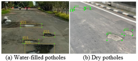
The dataset of road damage photographs used consists of images of roadways with water-filled potholes and dry potholes. The dataset is derived from Google sources, FixMystreet website, the Roboflow website and captured manually from Indonesian roads. The datasets taken and captured were selected from Indonesia, which were manually taken in East Java with all images taken during the day between 10 am and 1 pm. For datasets of dry potholes, it was carried out in the dry season, while for datasets of water-filled potholes it was carried out in the rainy season after the rain had stopped. There is a total of 4,756 photos used as a dataset. The dataset includes photos from various angles and lighting conditions, as well as photographs with varying hole sizes. Prior to processing, the photos are made to have the same 640×640 pixels size and format file type using the JPG format. There is a total of 4,756 photos used as a dataset, with the split of the dataset for training 70% (3,329 photos), for validation 15% (713 photos) and for testing 15% (714 photos). Figure 1 shows an example of the water-filled pothole dataset. The distribution of the dataset label is shown in Table 1.
Figure 1. Overview of dataset
Table 1. Dataset label distribution
|
Label |
Dataset Object |
Amount |
Percentage |
|
L00 |
Dry pothole |
2378 |
50% |
|
L01 |
Water-filled pothole |
2378 |
50% |
|
Total |
4756 |
100% |
|
2.2 Convolutional neural network model
CNN is a deep neural network that is often used for visual analysis. Neural networks are made up of multiple layers, each of which contains neurons with varying weights and biases that may be trained [23]. The TensorFlow Object identification aplication interface, is used in the modeling technique to facilitate prepocesing, training, and implementation of object identification models [24]. For this study, pre-trained model used for reduction in training time and stability performance because the model has been trained to detect many usual objects in real life [25]. In this paper, CNN and TensorFlow-based models named MobileNet SSD V2 used for vehicle detection on edge device Jetson Nano.
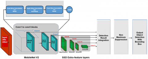
MobileNet SSD V2 is object detection model that contains 267 layers and 15 million parameters [26], providing inference in real-time using only edge device computing processes such as smartphones and Jetson Nano mini-computer. MobileNet SSD V2 actually consists of two models. The first one is the basic MobileNet V2 network with the SSD layer added. MobileNet is basically used as a backbone for the image classification process where the layer converts image pixels into features that describe the image [27]. Then the SSD layer is in charge of detecting the desired object by creating an object bounding box in an image [28]. As an illustration, the MobileNet SSD V2 structure can be seen in Figure 2 [29].
Figure 2. Structure of model MobileNet SSD V2
2.3 Edge device implementation
The implementation of edge device processing, as opposed to centralised server processing, is designed to enable real-time system responsiveness when integrated with the government monitoring framework. This approach ensures that road defects that occur on a given day can be detected immediately on that day. The centralised processing at government offices using servers can get a higher probability of processing queues, causing delays in analysing raw data from roads [30].
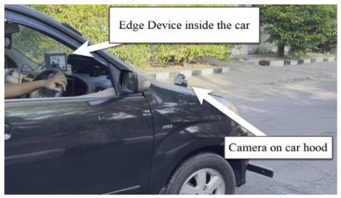
For this application, the Nvidia Jetson Nano with 4GB RAM was chosen as the leading device due to its compact form factor, efficient power consumption compatible with vehicle electrical systems using a cigarette lighter adapter, and its ability to effectively perform AI calculations [31]. In the system setup, the Jetson Nano is installed inside the vehicle, while the camera is mounted on the hood of the car, facing the road as shown in Figure 3.
Figure 3. Device implementation on vehicle
2.4 Testing scenario for optimized training model
To achieve optimal performance in detecting water-filled potholes on the road, it is essential to perform fine-tuning of the model configuration during training. The optimization process involves adjusting several hyperparameters to identify the best combination that maximizes detection accuracy while minimizing loss. In this study, the batch size and optimizer were varied across different configurations to optimize the training model. Batch size refers to the number of training samples—in this case, images—processed together in a single iteration before updating the model's weight parameters [32]. Batch sizes of 2, 4, 8, and 10 were tested. Training processes with batch sizes greater than 10 were terminated due to computational limitations. The optimizer is used during neural network training to adjust the model's weights and biases in order to minimize the loss function. This study employed two optimizers: Momentum optimizer and Adam optimizer [33]. A comprehensive overview of the testing scenarios for the optimized training model is presented in Table 2.
Table 2. Config and optimized training model scenario
|
Variables |
Testing Scenario |
|||
|
Model |
MobileNet SSD V2 |
|||
|
Num_classes |
2 |
|||
|
Num_steps |
25,000 |
|||
|
Learning_rate (lr) |
0.001 |
|||
|
Optimizer |
Momentum Optimizer |
Adam Optimizer |
||
|
Batch_size |
2 |
4 |
8 |
10 |
3.1 Result of training model
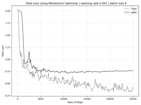
Before the model was implemented in edge device Jetson Nano. The model had to be trained and optimized using dataset that had been prepared. Model trained with the scenario like Table 2. To see the optimal and correct training results can be seen from several parameters. The first parameter is the total loss function. Total loss is divided into two training and validation. The smaller the training total loss the better which means the model learns to recognise objects better, but it must be balanced with a small validation total loss and not far from the training total loss [34]. Because the total loss validation indicates that in the training process when the model has recognised the object well and added a new object image dataset, the model can recognise it well, meaning that the total loss validation value still can follow the decrease in total loss training. If the opposite happens, it means that the model has memorised datasets and cannot recognise new datasets, it also called overfitting [35].
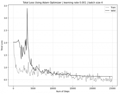
For the Momentum optimizer case in Figure 4, the observed divergence between decreasing training loss and increasing validation loss after 15,000 training steps clearly indicates overfitting. In comparison with Figure 5 using Adam Optimizer shows that the total loss validation can still follow the total loss training until the number of steps reaches 25,000.
Figure 4. Comparison results of total loss in training and validation using Momentum optimizer
Figure 5. Comparison results of total loss in training and validation using Adam optimizer
The second parameter to determine the good result of training is performance metrics. Based on the confusion matrix, the performance metrics test result used three variables in Eqs. (1)-(3).
Precision $=\frac{\text { True Positive }}{\text { True Positive }+ \text { False Positive }}$ (1)
Recall $=\frac{\text { True Positive }}{\text { True Positive }+ \text { False Negative }}$ (2)
F1 Score $=2 \times \frac{\text { Precision } \times \text { Recall }}{\text { Precision }+ \text { Recall }}$ (3)
Precision denotes the degree of accuracy between actual data and predicted data results produced by model. In other words, the proportion of detected data that is actually correct is measured. Recall describes the success of the model in retrieving information. In other words, the proportion of actual correct data that is detected is measured. The F1 score describes a metric combination of precision and recall. The formula uses the harmonic mean of recall and precision [36]. It is particularly useful in scenarios involving imbalanced datasets, where the distribution of classes is uneven. The formula itself provides a balanced metric between false positive and false negative. The metric accuracy is not utilized for model evaluation because it needs calculation of true negatives, which are not defined in object detection. For detecting objects in real life, the system focuses on identifying and localizing coordinate of objects within images, and there is no practical way to count the number of possible locations where no object is detected.
As a result, metrics such as precision, recall, and F1 score are preferred, as they do not depend on true negatives and provide a more meaningful assessment of model performance in detecting and localizing objects. For MobileNet SSD V2, after training automatically shows the performance metrics with the mean Average Precision (mAP), Average Recall (AR) and F1 score using Intersection over Union (IoU) at 0.5. IoU is the value used to compare the ground truth to the expected overlap bounding box. Table 3 shows the result model optimized with the selected scenario.
Table 3. Result model optimized selected scenarios
|
Optimizer Config |
Batch Size |
Total Loss |
Performance Metrics |
|||
|
Training |
Validation |
mAP |
AR |
F1 Score |
||
|
Momentum Optimizer lr=0.001 |
2 |
0.542 |
0.697 |
0.642 |
0.477 |
0.547 |
|
4 |
0.362 |
0.767 |
0.673 |
0.467 |
0.551 |
|
|
8 |
0.359 |
0.772 |
0.661 |
0.472 |
0.55 |
|
|
10 |
0.341 |
0.786 |
0.654 |
0.471 |
0.548 |
|
|
Adam Optimizer lr=0.001 |
2 |
0.4 |
0.647 |
0.617 |
0.488 |
0.348 |
|
4 |
0.679 |
0.628 |
0.68 |
0.508 |
0.582 |
|
|
8 |
0.415 |
0.7 |
0.667 |
0.484 |
0.561 |
|
|
10 |
0.345 |
0.732 |
0.675 |
0.471 |
0.554 |
|
Table 3 shows the result of selected scenario which is the optimizer and batch size. Out of 8 scenario in training model process, the highest F1 score occured in configuration using Adam Optimizer with learning rate 0.001, and the batch size using 4. The mAP obtained in 0.68, Average Recall (AR) in 0.508, and F1 score obtained in 0.582. When compared with previous research of road damage detection from Hernanda et al. [37], with the same model obtained the result of precision (mAP) in 0.0869, recall (AR) in 0.241 and F1 score not mentioned in the result. Despite the different sizes of datasets used and the label of road damage which is in that research including crack, the higher value of precision and recall obtained in this research.
For road damage surveys in Indonesia, one of the variables required in the survey is the number of potholes per 100 meters of road. For the application of real-world road damage surveys based on neural network automation technology, the precision value, recall value and especially the F1 score describe the detailed level accuracy of this technology in detecting the correct number of potholes. A precision of 0.68 implies that more than two-thirds of the detections are correct, a recall of 0.508 implies that the model identifies more than half of the actual potholes, and the F1 score can be used as a summary of the model's accuracy that a value of 0.582, means that the model when applied in the real world with the exactly number potholes and conditions as the training model dataset, the system model's accuracy is 58.2% in detecting potholes.
3.2 System performance testing in detection object on road
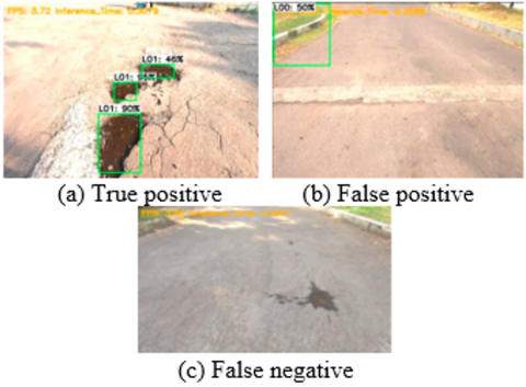
The system's detection performance where potholes are filled with water, is compared to its performance under dry conditions, where potholes on the same location in condition not filled with water. At the road site used for the research in Kertajaya Indah Street, Surabaya city, Indonesia, there were 37 potholes of 300 metres road. Despite the limited sample size that may limit the generalizability of finding, the research was conducted under realistic field condition using edge device system in a car, with still ensure diversity of pothole condition including variation of dimension, depth and the presence of the water in the pothole. At the road site used for the study, there were 37 potholes. Considering the weather conditions and site characteristics, the tests were conducted by deliberately filling the potholes with water. After that, data was collected, and performance was evaluated using the confusion matrix parameters: True Positive (TP), False Positive (FP), and False Negative (FN). True Positive in this test represents the circumstance where there is a pothole and the projected bounding box is correct. A false positive occurs when the projected bounding box is erroneous or does not correspond to the actual object label. A false negative occurs when there is a pothole but no projected bounding box. Definition of this matrix can be represented in Figure 6.
Figure 6. Matrix definition result
Then calculate the precision, recall and F1 score value from the matrix. A higher precision suggests fewer incorrectly classified objects as potholes. Recall describes the system's capacity to detect a large number of actual potholes. Higher recall implies the system will overlook fewer potholes. The F1 score is the fundamental metric for aessessing the system's accuracy, integrating precision and recall into a single score helpful for evaluating the precision-to-recall ratio. The testing procedure is computed for each Stationing (STA), a value used by road authorities to calculate the length of each 1 STA, which corresponds to 100 meters. This test covers a distance of 3 STA, or 300 meters with the speed of vehicle in 15 km/h. The first test, detecting dry potholes that the result shown in Table 4, then detecting water-filled potholes as comparison, the result shown in Table 5.
Table 4. System performance of detecting dry potholes
|
STA |
Num of Potholes |
TP |
FP |
FN |
Precision |
Recall |
F1 Score |
|
1 |
4 |
2 |
1 |
2 |
0.667 |
0.50 |
0.571 |
|
2 |
21 |
13 |
3 |
8 |
0.813 |
0.619 |
0.703 |
|
3 |
12 |
5 |
2 |
7 |
0.714 |
0.417 |
0.526 |
|
Total |
37 |
20 |
6 |
17 |
0.769 |
0.541 |
0.635 |
Table 5. System performance of detecting water-filled potholes
|
STA |
Num of Potholes |
TP |
FP |
FN |
Precision |
Recall |
F1 Score |
|
1 |
4 |
3 |
0 |
1 |
1 |
0.75 |
0.857 |
|
2 |
21 |
11 |
0 |
10 |
1 |
0.524 |
0.688 |
|
3 |
12 |
5 |
1 |
7 |
0.833 |
0.417 |
0.556 |
|
Total |
37 |
19 |
1 |
18 |
0.950 |
0.514 |
0.667 |
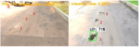
From Table 4 and Table 5, in overall STA of 300 metres road, the system has a tendency to get a precision value greater than the recall value, this illustrates that the system can minimise the identification of the bounding box of holes that are not actually holes. F1 score STA 1 in Table 4 get a lower value compared to water-filled pothole in Table 5. This may be due to the position of the pothole captured by the camera which cannot capture the pothole well as shown in Figure 7.
Figure 7. Comparison of the position potholes captured by the camera
The overall STA, system gets the best performance when detecting water-filled pothole with value Precision 0.95, Recall 0.514 and F1 score 0.667. Based on the F1 score, it can be interpreted that system can detect and classify 0.667 or 66.7% from the total potholes in that road.
3.3 System performance testing with vehicle speed function
The system for classification of water-filled potholes was tested, with the changing variable of vehicle speed. The speed used was constant on 15 km/h, 25 km/h, and 30 km/h. The testing was done on the same road as previous test.
Table 6. Testing result detection water-filled pothole with different vehicle speed
|
Speed (km/h) |
Num of Potholes |
TP |
FP |
FN |
Precision |
Recall |
F1 Score |
|
15 |
37 |
19 |
1 |
18 |
0.95 |
0.514 |
0.667 |
|
25 |
17 |
2 |
20 |
0.895 |
0.459 |
0.607 |
|
|
30 |
16 |
2 |
21 |
0.889 |
0.432 |
0.582 |
From Table 6, within a 300-meter road or 3 STA, the model's results vary with different vehicle speeds, impacting system performance. As the speed increases, the true positive value decreases, indicating a reduction in accurately detected potholes, while the false negative value rises, signifying numerous undetected potholes. At speeds of 25 km/h and 30 km/h, the false positive value increased compared to 15 km/h. After calculating precision and recall, it further strengthens the observation that the system is missing potholes, as the recall value is significantly lower than precision. Regarding the F1 score, the lowest speed, 15 km/h, obtains the highest F1 score of 0.667. As the speed increases, the F1 score gradually decreases, reaching 0.582 at 30 km/h.
The system performance decreased with increasing vehicle speed. First, increased vibrations in the vehicle occur when vehicle at a higher speed. This can blur the pothole objects, making them challenging for the system to detect. Second, the Jetson Nano implementing the SSD MobileNet V2 model processes frames during inference at an average of 3.5 frames per second (FPS), meaning the system processes 3 FPS. With increased speed, many frames will be skipped as the number of frames that can be processed decreases. Third, the impact of increasing vehicle speed, higher probability of over exposure or under exposure frame captured by the camera especially when lighting condition can be varied drastically like there are shadow from tree or building. The auto exposure camera doesn’t adapt fast enough in higher speed.
Based on the system performance test with varying speeds, the optimal implementation of the system is observed at a real-world speed of 15 km/h. To achieve good results at higher speeds, overall system performance improvement is required to increases the FPS produced by the device. Several solutions to mitigate issues at high speeds include using a stabilizer such as a gimbal on the camera to reduce motion blur, using a high dynamic range (HDR) camera to get details when the lighting is too bright or too dark, and utilizing the camera that can be adjusted adaptively for the exposure.
After conducting tests, analyzing data results, and implementing the system in this research, several conclusions have been drawn. The optimized model configuration is achieved with 25,000 steps, batch size 4, and learning rate 0.001, resulting in the smallest validation loss 0.628 and the largest F1 score of 0.582. For the performance testing, the system effectively detects water-filled potholes compared to dry pothole. For dry potholes, the system achieves precision 0.769, recall 0.541, and F1 score 0.635. When detecting water-filled potholes, the system achieves values with precision 0.95, recall 0.514, and F1 score 0.667. Furthermore, performance testing concerning varying vehicle speeds indicates that the optimal speed for the edge device performance’s system is an average speed of 15 km/h. At this speed, the system demonstrates precision 0.95, recall 0.514, and F1 score 0.667. However, higher speeds necessitate a larger FPS, with this system obtaining an average of 3.5 FPS. Recommendations include obtaining test locations with a larger number of potholes and longer roads, improved edge device hardware using more powerful GPU like Nvidia Jetson Xavier, using higher resolution of camera and adding more than one camera to get wider and better capture of potholes. In addition to further research, existing systems can be combined with laser-based systems such as Kumar's research [13] to improve the accuracy and validation of pothole types whether they are dry potholes or water-filled potholes. Another way that can be added to further research is to integrate the Lidar sensor into the existing system, when detected by the camera, the lidar sensor will collect precise profiling of pothole.
|
AR |
Average Recall |
|
FN |
False Negative |
|
FP |
False Positive |
|
FPS |
Frame per Second |
|
lr |
Learning Rate |
|
mAP |
Mean Average Precision |
|
STA |
Stationing |
|
SSD |
Single Shot Multibox Detector |
|
TP |
True Positve |
[1] Indah, P.R., NurulIstifadah, N. (2020). The infrastructure investment effect and transportation sector toward economic growth in Indonesia. Opción: Revista de Ciencias Humanas y Sociales, (27): 24.
[2] Bella, F., Calvi, A., D’Amico, F. (2012). Impact of pavement defects on motorcycles’ road safety. Procedia-Social and Behavioral Sciences, 53: 942-951. https://doi.org/10.1016/j.sbspro.2012.09.943
[3] Adianto, S., Mudjanarko, S.W. (2020). Study prone to traffic accidents on Diponegoro Street–Surabaya. IJTI: International Journal of Transportation and Infrastructure, 4(1): 50-61. https://doi.org/10.29138/ijti.v4i1.1165
[4] Setyawan, A., Febriayani, O., Handayani, F.S. (2023). Evaluasi nilai kondisi perkerasan jalan nasional dengan metode pavement condition index (PCI) (Studi kasus: Ruas Jalan Lingkar demak, Jalan Losari (Batas Prov. Jawa Barat)–Pejagan, dan Jalan Batas Kota Rembang-Bulu (Batas Prov. Jawa Timur)). Matriks Teknik Sipil, 11(1): 16-23. https://doi.org/10.20961/mateksi.v11i1.64685
[5] Kumalawati, A., Jhon, Y.E., Rizal, A.H. (2023). Faktor penyebab Kerusakan jalan pada ruas Jalan Pantura Kabupaten Ende dengan metode Pavement Condition Index (PCI). Jurnal Forum Teknik Sipil (J-ForTekS), 3(1): 65-74. https://doi.org/10.35508/forteks.v3i1.4695
[6] Mestuni, W.B., Hartatik, N. (2023). Road damage evaluation on rigid pavement with pavement condition index method in Klakah Rejo-Benowo road, Surabaya City, East Java. Jurnal Teknik Sipil, 23(4): 635-643. https://doi.org/10.26418/jts.v23i4.61048
[7] Yalew, L., Virgianto, G., Inagi, M., Tomiyama, K. (2023). Impact of a pothole on road user response in terms of driving safety and comfort for pavement maintenance prioritization. Journal of JSCE, 11(2): 23-21035. https://doi.org/10.2208/journalofjsce.23-21035
[8] Rana, P., Singh, R.R. (2018). Impact of rains on road transport. International Journal of Engineering Development and Research, 6(4): 97-100.
[9] Sukur, K.M., Nordin, R.M., Jaluddin, S.N., Yacob, R. (2023). Influence of poor drainage system on durability of the road pavement. AIP Conference Proceedings, 2888(1): 060003. https://doi.org/10.1063/5.0167960
[10] Khairunnisa, S.Z., Buana, C. (2023). Analisa kondisi dan perbaikan perkerasan pada ruas jalan Gresik–Paciran KM SBY 28 sampai dengan KM SBY 38 dengan menggunakan metode PCI dan SDI. Jurnal Teknik ITS, 12(1): E39-E45. https://doi.org/10.12962/j23373539.v12i1.114930
[11] Samsuri, S., Surbakti, M., Tarigan, A.P., Anas, R. (2019). A study on the road conditions assessment obtained from International Roughness Index (IRI): Roughometer vs Hawkeye. Simetrikal: Journal of Engineering and Technology, 1(2): 103-113. https://doi.org/10.32734/jet.v1i2.756
[12] Buana, C., Widyastuti, H., Prastyanto, C.A., Sudibyo, R.W. (2023). The effect of water below the road surface on surface distress index (SDI) values in the road condition survey (RCS) method. IOP Conference Series: Earth and Environmental Science, 1276(1): 012047. https://doi.org/10.1088/1755-1315/1276/1/012047
[13] Vupparaboina, K.K., Tamboli, R.R., Shenu, P.M., Jana, S. (2015). Laser-based detection and depth estimation of dry and water-filled potholes: A geometric approach. In 2015 Twenty First National Conference on Communications (NCC), Mumbai, India, pp. 1-6. https://doi.org/10.1109/NCC.2015.7084929
[14] Rani, M.R., Mustafar, M.Z.C., Ismail, N.H.F., Mansor, M.S.F., Zainuddin, Z. (2021). Road peculiarities detection using deep learning for vehicle vision system. IOP Conference Series: Materials Science and Engineering, 1068(1): 012001. https://doi.org/10.1088/1757-899X/1068/1/012001
[15] Garcillanosa, M.M., Pacheco, J.M.L., Reyes, R.E., San Juan, J.J.P. (2018). Smart detection and reporting of potholes via image-processing using Raspberry-Pi microcontroller. In 2018 10th International Conference on Knowledge and Smart Technology (KST), Chiang Mai, Thailand, pp. 191-195. https://doi.org/10.1109/KST.2018.8426203
[16] Lee, T., Chun, C., Ryu, S.K. (2021). Detection of road-surface anomalies using a smartphone camera and accelerometer. Sensors, 21(2): 561. https://doi.org/10.3390/s21020561
[17] Thompson, N.C., Greenewald, K., Lee, K., Manso, G.F. (2020). The computational limits of deep learning. arXiv preprint arXiv:2007.05558. https://doi.org/10.48550/arXiv.2007.05558
[18] Basulto-Lantsova, A., Padilla-Medina, J.A., Perez-Pinal, F.J., Barranco-Gutierrez, A.I. (2020). Performance comparative of OpenCV template matching method on Jetson TX2 and Jetson Nano developer kits. In 2020 10th Annual Computing and Communication Workshop and Conference (CCWC), Las Vegas, NV, USA, pp. 0812-0816. https://doi.org/10.1109/CCWC47524.2020.9031166
[19] Libutti, L.A., Igual, F.D., Pinuel, L., De Giusti, L., Naiouf, M. (2020). Benchmarking performance and power of USB accelerators for inference with MLPerf. In Proceedings of 2nd Workshop on Accelerated Machine Learning (AccML), pp. 1-15.
[20] Seshadri, K., Akin, B., Laudon, J., Narayanaswami, R., Yazdanbakhsh, A. (2021). An evaluation of Edge TPU accelerators for convolutional neural networks. arXiv preprint arXiv:2102.10423. https://doi.org/10.48550/arXiv.2102.10423
[21] Sandler, M., Howard, A., Zhu, M.L., Zhmoginov, A., Chen, L.C. (2018). Mobilenetv2: Inverted residuals and linear bottlenecks. In 2018 IEEE/CVF Conference on Computer Vision and Pattern Recognition, Salt Lake City, UT, USA, pp. 4510-4520. https://doi.org/10.1109/CVPR.2018.00474
[22] Kumar, A., Zhang, Z.J., Lyu, H. (2020). Object detection in real time based on improved single shot multi-box detector algorithm. EURASIP Journal on Wireless and Networking, 204. https://doi.org/10.1186/s13638-020-01826-x
[23] Alzubaidi, L., Zhang, J.L., Humaidi, A.J., Al-Dujaili, A. et al. (2021). Review of deep learning: Concepts, CNN architectures, challenges, applications, future directions. Journal of Big Data, 8: 53. https://doi.org/10.1186/s40537-021-00444-8
[24] Yoon, H., Lee, S.H., Park, M. (2020). TensorFlow with user friendly graphical framework for object detection API. arXiv preprint arXiv:2006.06385. https://doi.org/10.48550/arXiv.2006.06385
[25] Mtashre, A.K., Kareem, D.M., Muhsen, Z.A. (2024). Enhancing object detection techniques through transfer learning and pre-trained models. Journal of Engineering Sciences and Information Technology, 8(3): 40-52. https://doi.org/10.26389/AJSRP.K270724
[26] Lian, L., Mariano, V.Y. (2023). Recognition of traffic police gestures based on transfer learning. In 2023 3rd International Conference on Electronic Information Engineering and Computer Science (EIECS), Changchun, China, pp. 293-296. https://doi.org/10.1109/EIECS59936.2023.10435629
[27] Jin, L., Liu, G.D. (2021). An approach on image processing of deep learning based on improved SSD. Symmetry, 13(3): 495. https://doi.org/10.3390/sym13030495
[28] Ulaszewski, M., Janowski, R., Janowski, A. (2022). Application of computer vision to egg detection on a production line in real time. ELCVIA: Electronic Letters on Computer Vision and Image Analysis, 20(2): 113-143. https://doi.org/10.5565/rev/elcvia.1390
[29] Chiu, Y.C., Tsai, C.Y., Ruan, M.D., Shen, G.Y., Lee, T.T. (2020). Mobilenet-SSDv2: An improved object detection model for embedded systems. In 2020 International Conference on System Science and Engineering (ICSSE), Kagawa, Japan, pp. 1-5. https://doi.org/10.1109/ICSSE50014.2020.9219319
[30] Shi, W.S., Cao, J., Zhang, Q., Li, Y.H.Z., Xu, L.Y. (2016). Edge computing: Vision and challenges. IEEE Internet of Things Journal, 3(5): 637-646. https://doi.org/10.1109/JIOT.2016.2579198
[31] Sarvajcz, K., Ari, L., Menyhart, J. (2024). AI on the road: NVIDIA Jetson Nano-powered computer vision-based system for real-time pedestrian and priority sign detection. Applied Sciences, 14(4): 1440. https://doi.org/10.3390/app14041440
[32] Lin, R.Q., Yu, C.J., Han, B., Liu, T.L. (2023). On the over-memorization during natural, robust and catastrophic overfitting. arXiv preprint arXiv:2310.08847. https://doi.org/10.48550/arXiv.2310.08847
[33] Wilson, A.C., Roelofs, R., Stern, M., Srebro, N., Recht, B. (2017). The marginal value of adaptive gradient methods in machine learning. arXiv preprint arXiv:1705.08292. https://doi.org/10.48550/arXiv.1705.08292
[34] Masters, D., Luschi, C. (2018). Revisiting small batch training for deep neural networks. arXiv preprint arXiv:1804.07612. https://doi.org/10.48550/arXiv.1804.07612
[35] Bengio, Y. (2012). Practical recommendations for gradient-based training of deep architectures. In Neural Networks: Tricks of the Trade: Second Edition. Springer, Berlin, Heidelberg, pp. 437-478. https://doi.org/10.1007/978-3-642-35289-8_26
[36] Powers, D.M. (2020). Evaluation: From precision, recall and F-measure to ROC, informedness, markedness and correlation. International Journal of Machine Learning Technology, arXiv preprint arXiv:2010.16061. https://doi.org/10.48550/arXiv.2010.16061
[37] Hernanda, Z.S., Mahmudah, H., Sudibyo, R.W. (2022). CNN-based hyperparameter optimization approach for road pothole and crack detection systems. In 2021 IEEE World AI IoT Congress (AIIoT), Seattle, WA, USA, pp. 538-543. https://doi.org/10.1109/AIIoT54504.2022.9817316