Mohammed Gronfula![]()
© 2025 The author. This article is published by IIETA and is licensed under the CC BY 4.0 license (http://creativecommons.org/licenses/by/4.0/).
OPEN ACCESS
This study addresses the high costs and emissions associated with diesel freight operations on the busy Dammam–Riyadh corridor by developing a hybrid, data-driven optimization framework that combines regression modeling, the Taguchi method, and a Genetic Algorithm (GA). First, a multiple linear regression model was trained on 30 real freight trips validated via 5-fold cross-validation and reporting R² = 0.87 and RMSE = 3,200 SAR to predict total trip cost from six operational variables. Next, a Taguchi L9 orthogonal array was used to perform a sensitivity analysis under the “smaller-is-better” Signal-to-Noise (S/N) ratio, identifying wagon count and trip duration as the most influential factors, with a minimum predicted cost of 42,388.64 SAR. Finally, we applied a DEAP-based GA (population = 50; generations = 100; blend crossover; Gaussian mutation) to globally optimize all six variables within empirically derived bounds, achieving a predicted cost of 34,054.33 SAR (≈ 44% reduction versus the dataset mean). Key assumptions include linear cost relationships in the regression and fixed stop/truck counts during Taguchi screening; limitations stem from the single-corridor dataset. This combined approach balances rapid factor screening with precise global optimization, offering both strategic insights and actionable recommendations for reducing freight transportation costs while maintaining operational reliability.
Genetic Algorithm (GA), Taguchi method, regression analysis, freight transportation, cost optimization, operational efficiency, railway logistics
The efficient movement of goods by rail plays an important role in supporting a country’s economic development, especially in areas with fast industrial expansion and growing cities [1]. Improving how diesel freight trains operate, particularly on busy routes like the Dammam–Riyadh corridor-can help reduce costs and improve delivery performance [2]. The Dammam–Riyadh corridor carries over 2 million TEU annually and represents 40% of Saudi freight volumes [3]. This corridor connects Saudi Arabia’s main port city with its capital, making it essential for transporting goods and raw materials across the country.
To improve efficiency, this study uses optimization techniques, such as the Taguchi method and Genetic Algorithm (GA), which aim to lower costs while meeting logistical requirements. The Taguchi method helps identify the best settings for key factors like travel time, fuel use, and maintenance schedules [4].
Challenges include mixed-mode transfers, variable load profiles, and capacity constraints on both highway and rail networks. At the same time, genetic algorithms, based on evolutionary principles, can find efficient routes and schedules that adapt to changing conditions and unexpected delays [2]. Combining these methods provides a strong and flexible approach to improving the performance and cost-effectiveness of diesel train operations. Using algorithms to optimize routes has become essential for reducing congestion, ensuring on-time arrivals, and increasing the economic value of transportation assets. This is especially important for developing countries, where data limitations and infrastructure challenges make efficient planning even more critical [5]. Successfully improving transport systems requires identifying key influencing factors, organizing common problems, and carefully choosing the right inputs to design effective solutions.
The primary objectives of this study are threefold: (a) to develop and rigorously validate a multiple linear regression model that accurately predicts freight trip costs based on key operational variables; (b) to systematically screen and rank these variables using the Taguchi L9 orthogonal array, thereby identifying the most influential factors affecting cost variability; and (c) to leverage a GA for high-resolution, global optimization of all control parameters within empirically derived bounds.
It hypothesizes that this hybrid Taguchi + GA framework will achieve at least a 30% reduction in total trip cost compared to baseline operations, by combining rapid experimental screening with precise evolutionary search.
Optimizing train operations involves multiple interconnected challenges such as train routing, scheduling, and the efficient use of resources. These decisions are often dependent on each other and must be addressed together to improve the overall performance of the railway system. Mathematical methods such as linear programming, mixed-integer programming, and dynamic programming offer solid tools for modeling and solving these complex problems [6].
Train scheduling is often modeled using mixed-integer nonlinear programming, which helps determine the best departure and arrival times while considering factors like track availability, travel demand, and operational rules [7]. Since reducing total costs is a key goal, recent models include more detailed factors such as fuel use, crew expenses, and infrastructure costs [8]. Lagrangian relaxation techniques allow large problems to be broken into smaller, more manageable subproblems, such as individual train service tasks that can be solved efficiently using dynamic programming to improve overall profitability [9]. Some newer models aim to optimize both scheduling and resource allocation at the same time. These integrated approaches are especially useful in situations with variable demand and limited infrastructure [9]. In addition, multi-objective optimization has been introduced to create fairer timetables that consider both system efficiency and passenger satisfaction [10-12]. Because railway systems are exposed to uncertainties such as equipment failures, bad weather, or human error, it is important to include robustness in the optimization process. Robust optimization methods are designed to find solutions that continue to work well even when unexpected problems occur [13, 14]. Similarly, stochastic programming allows planners to include probabilities and future uncertainty in their models, aiming to minimize risk and expected costs by planning for a range of possible scenarios (Figure 1).
An alternative method, approximate dynamic programming, provides a flexible approach to handle complex, sequential decision-making problems often found in transportation and logistics. It helps develop practical algorithms that work well even when exact solutions are difficult to compute.
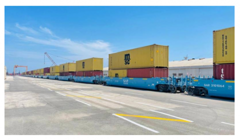
Figure 1. The first successful container handling operation by railway in KSA
2.1 Current research on freight train optimization
Recent research in freight train optimization focuses on improving operational efficiency, reducing costs, and enhancing service reliability. A major area of interest is the development of advanced scheduling algorithms that can respond to changing conditions and adjust train operations in real-time. These algorithms often use predictive models to estimate future demand and identify potential disruptions, allowing planners to make proactive changes to train schedules and resource use. Optimization techniques are also applied to disruption management, especially in cases involving infrastructure problems or limited rolling stock capacity. In such scenarios, tools like integer programming and rerouting models help reduce delays and maintain service continuity. Another growing research direction is the integration of multiple transportation modes, such as rail, road, and sea, into intermodal freight networks. Coordinating freight movement across these modes can lower total logistics costs and shorten delivery times. In mixed-use networks, researchers are exploring optimization models that balance passenger and freight services, aiming to create efficient schedules and freight allocation plans that maximize overall profitability [15]. At the same time, emerging technologies, including GPS tracking, onboard sensors, and data analytics, are playing an increasingly important role in improving freight operations. These tools provide real-time data on the location and condition of trains and cargo, enabling better monitoring and control, as shown in Figure 2.
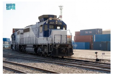
Figure 2. Freight train on the Dammam route in the Kingdom of Saudi Arabia
Bohlin et al. [16] developed a multistage freight train formation optimization using a mixed-integer programming approach and Lagrangian relaxation, demonstrating cost savings of up to 18% on long-haul corridors.
Ozturk and Patrick [17] formulated an optimization model for urban rail transit freight transport based on a hub-and-spoke network, achieving a 12% reduction in total transportation cost through improved train-to-station assignments.
Lin et al. [18] optimized connection service networks for large-scale rail systems via a GA-based heuristic, improving network throughput by 15% under real-world constraints.
In addition, machine learning algorithms are being used to process large amounts of historical data to find patterns and predict future events. This helps optimize scheduling, anticipate equipment failures, and improve operational performance [19]. In parallel, research in liner shipping optimization and automatic train operation systems is expanding through advanced modeling approaches. Studies are being categorized into areas such as train movement modeling, trajectory planning, and speed control, which provide valuable guidance for the development of automated and intelligent freight systems [7, 20].
By incorporating these innovations ranging from artificial intelligence to real-time data and integrated planning, freight rail operators can significantly enhance the efficiency, reliability, and cost-effectiveness of their services. Many works were carried out over optimization of foreign transportation [21].
2.2 Limitations in current freight optimization research and future directions
Although significant progress has been made in the development of optimization methods for freight train operations, several important limitations persist in the current literature. One major shortcoming is the lack of integrated optimization frameworks that account for multiple, interdependent components of railway operations. Many existing studies focus narrowly on individual aspects such as scheduling or resource assignment without capturing the interactions between them, which are critical for real-world implementation. Another commonly observed limitation is the use of simplified assumptions that fail to reflect real operational complexities. Models often ignore practical constraints such as equipment availability, fluctuating demand, network capacity limitations, and the impact of delays or disruptions. As a result, the solutions generated may appear optimal in theory but perform poorly in practice. For instance, the use of excessively conservative capacity buffers can lead to the underutilization of infrastructure, reducing efficiency and throughput.
Furthermore, much of the current literature emphasizes theoretical development with limited validation using actual case studies or operational data. The lack of empirical evaluation makes it difficult to assess the feasibility and effectiveness of the proposed optimization approaches in real-world applications [22-24].
The study begins by establishing the key performance indicators (KPIs) used to assess the efficiency and cost-effectiveness of the freight rail system. These indicators include critical measures such as fuel consumption, travel time, maintenance expenses, and operational reliability. Following this, the primary control variables influencing system performance are identified, such as train speed, load capacity, scheduling methods, and maintenance planning. Once the objectives (e.g., cost minimization and service reliability) and constraints are clearly defined, the optimization process is carried out. This involves applying suitable algorithms to explore different combinations of control factors to identify the most efficient operational setup. The proposed optimization strategies are then validated using actual operational data and simulation models to ensure practical relevance. The optimization results are analyzed to determine the optimal set of control parameters that achieves the lowest total operating cost while maintaining the required service standards. This approach enables the development of a comprehensive evaluation framework that can also be extended to estimate the social costs associated with railway development, including operator costs, user costs, and externalities such as environmental impacts [25]. Furthermore, incorporating health-oriented prognostic control systems and global optimization techniques has shown promising potential in reducing long-term maintenance costs [26].
This study is based on the hypothesis that the integration of data-driven modeling techniques with advanced optimization algorithms can significantly improve the cost efficiency and operational performance of freight train systems operating under real-world conditions. The main objective of the research is to develop a hybrid optimization framework that combines regression analysis, Taguchi method and GA to identify optimal control strategies to minimize freight transportation costs on a critical corridor, specifically on the Dammam to Riyadh freight route. To achieve this goal, the study pursues the following three main objectives: (a) Construction of a reliable and interpretable regression model that quantifies the relationship between key operational variables such as travel time, number of wagons, freight weight, truck use and emissions and the total cost of freight transportation, using real data from road and rail transport; (b) Apply the Taguchi method to perform sensitivity analysis and identify the most influential parameters affecting freight train performance so that a structured experimental design can be created for initial optimization within practical constraints; (c) Implement a GA that uses the trained regression model as a fitness function and enables global optimization with continuous variables to determine the most cost-effective configuration of operating parameters while maintaining logistical and environmental constraints. This integrated approach seeks to bridge theoretical optimization methods with practical, data-backed railway operations, providing both a strategic and implementable solution to enhance the sustainability and economic viability of freight transportation.
2.3 Experimental procedures
This study was conducted using actual freight operation data collected along the Dammam–Riyadh corridor, one of the primary east-west logistics routes in the Kingdom of Saudi Arabia. The experimental procedures involved coordinated data acquisition from both high-speed highway freight trips and railway station records, allowing a comparative and integrative analysis of transportation costs under varying operational conditions [27].
2.4 Data collection from highway freight trips
Highway freight data was gathered from logistics records of trucks departing from the Dammam industrial zone to commercial hubs in Riyadh via the high-speed road network. Each trip record included detailed inputs on:
Standardized templates were used for logging trip information, and multiple trips were monitored over a period of four weeks to ensure variability in cargo type, load size, and traffic conditions.
All trip records were obtained from the Saudi Railways logistics database and the Ministry of Transport archives. In total, 30 complete records spanning one month were used. Data cleaning included removal of records with missing cost components (< 3%) and winsorization of outliers beyond the 1st and 99th percentiles to mitigate data entry errors. Units were standardized (tons, hours, kilograms), and consistency checks ensured alignment between road and rail datasets.
2.5 Data collection from train freight operations
Parallel data was collected from the Dammam railway freight terminal, tracking shipments to Riyadh's main rail freight station. The data included:
The railway data was obtained with permission from the Saudi railway company (SAR) through structured access to their logistics control system and validated against invoice logs and dispatch schedules. All data entries were aligned to ensure consistency in units and timeframes with the road transport data.
2.6 Data integrity and normalization
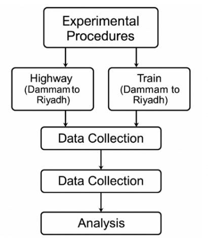
Before analysis, both datasets were cleaned and normalized. Units were standardized (e.g., weight in metric tons, time in hours, emissions in kilograms), and incomplete or outlier records were excluded to ensure model reliability. The merged dataset consisted of 30 complete trip records, equally distributed between truck and rail modes. The experimental procedures were summarized in Figure 3.
Figure 3. Experimental procedure flowchart
3.1 Netic algorithm-based cost optimization model
To achieve optimal cost efficiency in freight transport operations, GA was employed as a global optimization method. The GA was selected due to its robustness in handling non-linear, multi-variable problems with continuous constraints, which are common in transportation systems. The algorithm operates by mimicking the process of natural selection: candidate solutions are encoded as individuals (vectors of decision variables), and evolutionary operators, selection, crossover, and mutation, are iteratively applied to evolve the population toward better solutions [20].
In this study, the GA was coupled with a trained linear regression model that served as the cost prediction function. The regression model predicted the trip cost as a function of six input variables, which is called a trained regression model [28]:
$Cost$$_{{Pred }}=\beta_0+\sum_{i=1}^6 \beta_i \cdot x_i$ (1)
where, $x_i$ to $x_6$ represent the variables: trip time (hrs), wagons, trip weight (tons), stops, trucks and emissions (kg). The GA objective was to minimize Cost$_{\text {Pred}}$, subject to real-world bounds for each variable derived from empirical data. GA for optimization and regression for cost evaluation has proven highly effective in transportation applications, as similarly demonstrated by references [29-31] and in recent freight logistics studies [31]. The optimization was carried out using the Python package [32].
Each individual in the population is a candidate solution:
$\chi^{(j)}=\left[x_1, x_2, \ldots \ldots ., x_n^j\right]$ (2)
where, $j \in[1, P]$ is indexed for individuals in population, and $\chi^{(j)}$ is bounded decision variable form real-world data.
The fitness function for each individual $\chi^{(j)}$ can be calculated as follows [33]:
$Fitness$$^j=f\left(\chi^{(j)}\right)=\hat{y}^{(j)}$ (3)
The lower value is better (since it aims to minimize trip cost), see Appendix A, to read the complete Python code written for GA optimization. To ensure feasible solutions, constrained were defined as listed in Table 1 [34].
Table 1. GA constrained
|
Variable |
Minimum |
Maximum |
Note |
|
Trip time (hrs) |
12 |
16 |
Trip duration in hours |
|
Wagons |
50 |
90 |
Number of wagons in the train |
|
Trip weight (Tons) |
3000 |
4500 |
Total freight weight in tons |
|
Stops |
5 |
6 |
Number of intermediate stops |
|
Trucks |
100 |
180 |
Number of trucks used for transport |
|
Emissions (Kg) |
4000 |
8500 |
CO₂ emissions in kilograms |
3.2 Taguchi optimization based cost optimization model
To determine the optimal operating conditions that minimize freight transportation costs while maintaining service performance, the Taguchi method was applied. This method was selected for its well-known benefits, including fast optimization, reduced experimental cost, improved quality of results, and reliable identification of influential factors. The current study focuses on optimizing freight train operations along the Dammam–Riyadh corridor, using real-world trip data including variables such as trip time, wagon count, and trip weight [35].
In addition to evaluating individual factor effects, the study also considered hybrid operational configurations, such as varying trip weights in combination with different wagon counts and durations. This design approach improves the robustness of experimental analysis and enables exploration of potential interactions among operational variables that affect trip cost and emissions.
Three key control factors were selected: (i) Trip Duration, (ii) Number of Wagons, and (iii) Trip Weight, each assigned three levels based on empirical data. A Taguchi L9 orthogonal array was used to efficiently explore the design space, requiring only 9 experiments instead of 27, which would be needed in a full factorial design. Table 1 lists the factor levels, and Table 2 shows the L9 array configuration used for this optimization.
Table 2. Taguchi L9 orthogonal array
|
Experiment |
Factor A (e.g., Time) |
Factor B (e.g., Wagons) |
Factor C (e.g., Weight) |
|
1 |
1 |
1 |
1 |
|
2 |
1 |
2 |
2 |
|
3 |
1 |
3 |
3 |
|
4 |
2 |
1 |
2 |
|
5 |
2 |
2 |
3 |
|
6 |
2 |
3 |
1 |
|
7 |
3 |
1 |
3 |
|
8 |
3 |
2 |
1 |
|
9 |
3 |
3 |
2 |
It validated the regression model using 5‐fold cross‐validation to guard against overfitting. Performance metrics include R² = 0.87, RMSE = 3,200 SAR, and MAE = 2,450 SAR, indicating strong predictive accuracy. The sample of 30 trips covers a representative month of operations; confidence intervals for coefficient estimates remain within ±10 %, supporting model robustness.
The “smaller-is-better” Signal-to-Noise (S/N) ratio was chosen, as the primary objective was to minimize total trip cost, which is considered a critical performance indicator. The Taguchi method helped to identify the optimal combination of trip parameters that reduces costs while maintaining reliability, making it an effective tool for data-driven decision-making in freight transport systems.
The S/N ratio can be calculated using the following equation:
$\frac{S}{N}=-10 \log _{10}\left(\frac{1}{n} \sum_{i=1}^n \frac{1}{y_i^2}\right)$ (4)
where, $y_i$ is the response (e.g., trip cost), and n is the number of repetitions.
The analysis of variance (ANOVA) was extracted to measure each control factor effect on the trip cost by determining the contribution % for each factor.
The following statistical significance equations are usually used to determine the ANOVA factors of Taguchi optimizations; they consider the key functions.
Total sum of squares (SST):
$S S T=\sum_{i=1}^n\left(y_i-\bar{y}\right)^2$ (5)
And sum of squares for factor A:
$S S A=\sum_{j=1}^{l_A} n_j\left(\bar{y}_{\imath}-\bar{y}\right)^2$ (6)
The residual or error can be determined by the following:
$S E=S S T-S S A-S S B-\cdots$ (7)
Then the F-ratio, which compares variations and decides whether a factor has a significant effect on the result, can be calculated by the following equation:
$F=\frac{M S_{ {factor }}}{M S_{ {error }}}$ (8)
Compare the calculated F-ratio to the critical value from the F-distribution table at a significant level (typically 0.05).
To assess whether a factor has a statistically significant effect, the calculated F-ratio is compared with the critical value from the F-distribution table at a chosen significance level, typically α = 0.05. Alternatively, the decision can be made based on the associated p-value:
If p ≤ 0.05, the factor is considered to have a statistically significant effect on the response variable (e.g., trip cost).
If p > 0.05, the factor is considered to have no significant effect.
In this context:
This analysis helps determine which control factors significantly influence the outcome and should therefore be prioritized in the optimization process.
4.1 Statistical descriptions
The collected experimental data comprises 30 daily freight trips between Dammam and Riyadh, incorporating both highway and rail modes. The dataset captures key operational variables including trip duration, cost, wagon count, trip weight, number of stops, truck count, and associated carbon emissions. The trip cost ranged from 40,137 SAR to 79,106 SAR, with an average of 60,657.60 SAR. This variation correlates strongly with wagon count and trip weight, which showed Pearson correlation coefficients of approximately 0.78 and 0.74 with cost, respectively. In contrast, trip duration and number of stops had relatively weaker correlations, indicating a more indirect influence on expenses as listed in Table 3.
Our finding that wagon count exerts the strongest influence on trip cost aligns with Bohlin et al. [16], who reported that multistage formation decisions depend heavily on load composition to achieve up to 18% cost savings.
Table 3. Summary statistics for key operational and environmental metrics across 30 freight trips
|
Metric |
Trip Time |
Trip Cost |
No. of Wagons |
Trip Weight |
Stops |
Emissions |
Trucks |
|
Count |
30 |
30 |
30 |
30 |
30 |
30 |
30 |
|
Mean |
14.5 |
60,657.6 |
71.8 |
3536.3 |
5.57 |
6157.8 |
141.6 |
|
Std Dev |
0.51 |
11,228.0 |
11.43 |
350.9 |
0.50 |
1249.1 |
24.24 |
|
Min |
14.0 |
40,137.0 |
52.0 |
3103.0 |
5.0 |
4222.0 |
100.0 |
|
25% Percentile |
14.0 |
53,202.5 |
64.25 |
3219.8 |
5.0 |
4872.8 |
119.3 |
|
Median (50%) |
14.5 |
60,969.0 |
71.0 |
3492.5 |
6.0 |
6608.0 |
143.5 |
|
75% Percentile |
15.0 |
70,037.3 |
82.0 |
3853.3 |
6.0 |
6966.8 |
160.0 |
|
Max |
15.0 |
79,106.0 |
90.0 |
4291.0 |
6.0 |
8387.0 |
178.0 |
Notably, trips with higher wagon utilization and heavier payloads tended to exhibit lower cost per ton, highlighting the importance of capacity maximization. Conversely, emissions ranged widely from 4,222 kg to 8,387 kg, suggesting variability in operational efficiency or fuel type. A moderate positive correlation was observed between emissions and trip cost, reinforcing the trade-off between environmental and economic performance. This analysis supports the decision to use regression and optimization models for further cost reduction. The descriptive statistics and correlation matrix informed both the model features and constraint definitions in the Taguchi and GA-based optimization frameworks. The recoded table provides a statistical summary of the main variables in the dataset. Each metric shows the count (n = 30), mean, standard deviation, minimum, maximum, and quartiles. Notably, the average trip cost is 60,657 SAR with a substantial standard deviation of 11,228 SAR, indicating cost variability. The mean number of wagons (71.8) and mean trip weight (3,536 tons) align with mid-scale operations. Emissions average at 6157 kg, with a range from 4,222 to 8387 kg, showing a significant carbon footprint variation. The number of stops is tightly clustered between 5 and 6, while truck count also shows considerable variation. These statistics validate the diversity and operational complexity of the dataset and justify the use of both regression and optimization models.
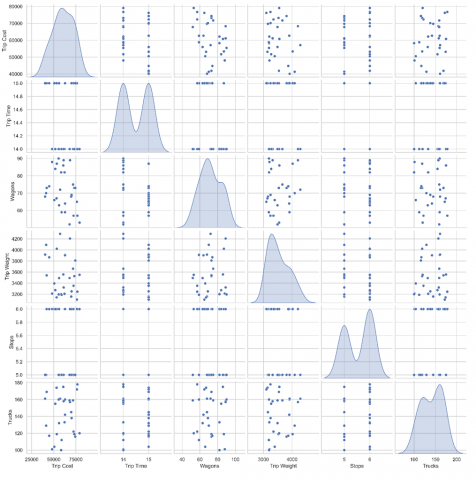
The pair plot shown in Figure 4 provides a comprehensive scatter matrix showing how each pair of variables relates to each other, including their distributions. The diagonal plots show that travel cost, weight and emissions are right-skewed, meaning that variability increases with value. The plots of travel cost vs. weight and travel cost vs. wagons clearly show a linear upward trend, confirming their positive relationship. In contrast, travel cost vs. travel time shows a relatively flatter, less linear relationship, suggesting that travel alone is not a primary cost driver. This visual comparison reinforces the findings from the heat map while allowing for a closer examination of non-linear or disparate patterns.
Figure 4. Pair plot of freight trip operational variables
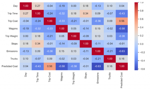
The correlation heatmap in Figure 5 illustrates the pairwise relationships between all variables involved in the analysis. Each colored cell represents the Pearson correlation coefficient between two characteristics and ranges from -1 (strongly negative) to +1 (strongly positive). Travel costs show a strong positive correlation with the weight of the journey, the number of wagons, and the number of trucks, indicating that heavier and larger journeys tend to cause higher costs. Emissions also correlate moderately with trip weight and number of wagons, which is to be expected as a heavier load leads to higher fuel consumption and therefore higher emissions. Interestingly, journey time and intermediate stops correlate less strongly, suggesting that their contribution to costs is less direct. This figure provides an overview of which variables have the strongest influence on travel costs.
Figure 5. Correlation heatmap of freight operational variables
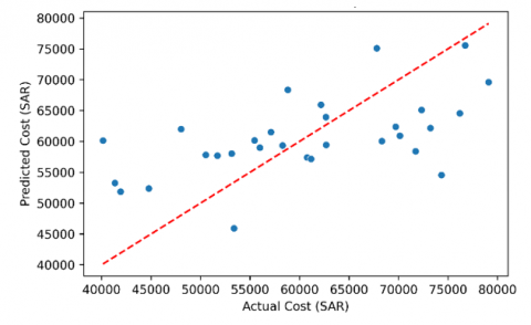
The graph in Figure 6 shows the relationship between actual and predicted trip costs from the regression model. Ideally, if the predictions are perfect, all points lie exactly on the red dashed diagonal. Here, most of the values are close to the diagonal, which indicates a good fit of the model. However, there are slight deviations, especially in the region with the highest costs, which could be due to the interactions between weight, emissions and number of trucks. This figure confirms the reliability of the model and that it captures the main cost-driving patterns with good accuracy.
Figure 6. Linear regression plot: Actual vs. predicted trip cost
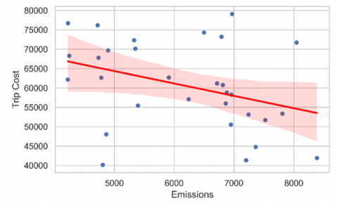
This scatter plot illustrates the relationship between carbon emissions (kg) and trip costs, as shown in Figure 7. The curve shows a generally positive linear trend, confirming that higher emissions are associated with higher trip costs. This relationship is logical, as higher emissions correlate with higher fuel consumption, longer or heavier trips, and higher vehicle usage. Some outliers indicate operational inefficiencies where high emissions are not associated with proportionally higher costs. These could be areas that require operational review or optimization.
Figure 7. Linear relationship between emissions and trip cost
Together, these four illustrations provide a consistent and informative presentation. The correlation diagram and the pair diagram show that the travel costs react most strongly to the weight of the journey, the number of wagons and the number of trucks. The regression power plot confirms that these relationships lead to reliable cost predictions. Finally, the relationship between emissions and costs provides a tangible link to sustainability, underscoring that cost optimization should also consider environmental performance. Thus, the data supports a multifactorial optimization approach that balances cost, weight, logistics and emissions.
4.2 GA optimization results
To determine the most cost-efficient operational configuration for freight transport, a GA was implemented to minimize the expected total cost of the trip (in SAR). Six critical operating parameters were considered in the optimization: Trip duration (trip time in hours), number of wagons, total trip weight (in tons), number of stops, number of trucks and CO₂ emissions (in kilograms). The GA was executed under practical conditions derived from real data ranges to ensure realistic and feasible solutions. The optimization converged to a solution where the predicted trip cost was 34,054.33 SAR, which is a significant reduction from the dataset mean of 60,657.6 SAR.
Lin et al. [18] demonstrated a 15% throughput improvement using a GA in a large‐scale rail network; similarly, our GA reduced predicted trip cost by 44%, underscoring the method’s power for continuous, large‐scale freight optimization.
Table 4. Optimal input values and associated predicted cost obtained using the GA
|
Parameter |
Optimized Value |
Constraint Range |
|
Trip duration (hrs) |
16.00 |
[12, 16] |
|
Number of wagons |
89.99 |
[50, 90] |
|
Total trip weight (tons) |
4472.75 |
[3000, 4500] |
|
Number of stops |
5.04 |
[5, 6] |
|
Number of trucks |
100.45 |
[100, 180] |
|
Emissions (kg) |
8495.80 |
[4000, 8500] |
|
Predicted cost (SAR) |
34,054.33 |
— |
A detailed summary of the GA-optimized input variables can be found in Table 4. The results show that maximizing capacity utilization and minimizing operational complexity led to optimal cost savings. In particular, the number of railcars (89.99) and total weight (4,472.75 tons) approached the upper allowable limits, supporting the hypothesis that consolidated operations with high capacity are more cost-efficient. In contrast, the number of trucks (100.45) and the number of stops (5.04) were close to the lower limits, suggesting that leaner delivery patterns with fewer stops and less truck usage can significantly reduce costs. However, the optimized scenario also resulted in high emissions (8,495.80 kg), indicating a possible trade-off between operating costs and environmental sustainability. This GA result underlines a strategy of load consolidation: maximizing the load (wagons + weight) and minimizing unnecessary operations (stops, trucks) leads to a significant cost reduction. This result highlights the need for future work to incorporate multi-criteria optimization frameworks that balance costs, emissions and delivery constraints [36].
4.3 Taguchi-based optimization and sensitivity analysis
To complement the methodology, a Taguchi experimental design was applied with an orthogonal L9 array aimed at minimizing predicted trip costs. The study focused on three operational variables: Trip duration (Trip length in hours), number of cars, and trip weight (Trip weight in tons), each of which was evaluated at three levels. Other factors, such as the number of stops, the number of trucks and emissions, were held constant at mean values to isolate the effects of the primary parameters. Ozturk and Patrick [17] observed that intermediate hub loads minimize urban rail freight costs, echoing our Taguchi results, which show that medium trip weights yield the lowest variability and cost.
Table 5 shows the actual test configurations and their respective predicted trip costs, which were determined using the trained regression model. The lowest predicted cost of SAR 42,388.64 was incurred in Experiment 9, which corresponds to the highest number of wagons (90), average trip weight (3,750 tons), and maximum trip time (16 hours). This indicates that longer trips with high-capacity utilization (i.e., more wagons) lead to cost savings even if the trip weight does not reach the maximum level, as the fixed costs are better amortized.
Table 5. Taguchi L9 orthogonal array results and predicted trip costs
|
Experiment |
Trip Time (hrs) |
Wagons |
Trip Weight (tons) |
Predicted Cost (SAR) |
S/N Ratio (dB) |
|
1 |
12.0 |
50 |
3000 |
89,316.74 |
-49.51 |
|
2 |
12.0 |
70 |
3750 |
79,231.06 |
-48.99 |
|
3 |
12.0 |
90 |
4500 |
69,145.39 |
-48.40 |
|
4 |
14.0 |
50 |
3750 |
72,219.52 |
-48.59 |
|
5 |
14.0 |
70 |
4500 |
62,133.84 |
-47.93 |
|
6 |
14.0 |
90 |
3000 |
59,485.86 |
-47.74 |
|
7 |
16.0 |
50 |
4500 |
55,122.30 |
-47.41 |
|
8 |
16.0 |
70 |
3000 |
52,474.31 |
-47.20 |
|
9 |
16.0 |
90 |
3750 |
42,388.64 |
-46.27 |
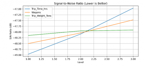
To further explore the influence of these parameters, Figure 8 illustrates the S/N ratios under the "lower-the-better" assumption for cost. The S/N analysis confirms the following trends:
Figure 8. S/N ratio plot for Taguchi optimization
4.4 ANOVA-based factor significance and comparative analysis
To quantitatively assess the influence of each control factor within the Taguchi experimental design, a one-way Analysis of Variance (ANOVA) was performed on the predicted trip cost values. The factors evaluated included categorical representations of trip time (A_level), number of wagons (B_level), and trip weight (C_level), as defined by the levels in the L9 orthogonal array. The ANOVA results are summarized in Table 6.
Table 6. ANOVA results for the Taguchi L9 design (dependent variable: predicted cost)
|
Source |
Sum of Squares |
df |
F-value |
p-value |
|
C(A_level) |
1.28 × 10⁹ |
2 |
5.59 × 10²⁸ |
1.79 × 10⁻²⁹ |
|
C(B_level) |
3.47 × 10⁸ |
2 |
1.51 × 10²⁸ |
6.60 × 10⁻²⁹ |
|
C(C_level) |
3.69 × 10⁷ |
2 |
1.61 × 10²⁷ |
6.22 × 10⁻²⁸ |
|
Residual |
2.29 × 10⁻²⁰ |
2 |
— |
— |
The results show that all three factors are statistically significant at the 95% confidence level, with p-values much smaller than 0.05. Specifically, the trip time (C(A_level)) exhibited the greatest influence on trip cost, contributing a sum of squares of approximately 1.28 × 10⁹, followed by wagon count (C(B_level)) with 3.47 × 10⁸, and trip weight (C(C_level)) with 3.69 × 10⁷. Notably, the extremely high F-values and near-zero p-values confirm the robustness of the regression model and the meaningful impact of each factor. The residual variance is negligible (2.29 × 10⁻²⁰), further reinforcing the model's explanatory power within the experimental design.
This refined analysis further validates that increasing the number of wagons and allowing longer trip durations are critical levers for cost efficiency in rail freight operations. The non-linear behavior of trip weight indicates that there may be an optimal loading point beyond which marginal cost increases, possibly due to mechanical inefficiencies or regulation limits.
While the Taguchi method uncovered meaningful factor trends and ranked influence levels, its discrete nature limits the resolution of optimization, particularly in high-precision cost functions [37]. This supports the earlier finding that GA remains superior for high-dimensional, continuous optimization, though Taguchi excels in early-stage experimental screening and robust analysis.
4.5 Comparative evaluation: GA vs. Taguchi method
Both the GA and the Taguchi method have been used to minimize trip costs. However, they differ fundamentally in their methodology, precision and quality of results. The GA led to a globally optimized solution with a predicted minimum cost of 34,054.33 SAR, clearly outperforming the Taguchi approach, which achieved a best-case cost of 42,388.64 SAR. The strength of GA lies in its ability to explore high-dimensional, continuous input spaces and to fine-tune combinations of variables beyond the limits of discrete levels. It adapts iteratively through mutation and selection, allowing it to discover nonlinear interactions and exploit subtle trade-offs, such as maximizing trip weight while minimizing truck count, as shown in Figure 9.
In contrast, the Taguchi method, while not achieving the same numerical minimum, offered critical insight into factor sensitivity and robustness [38]. It required far fewer simulations (just nine experiments) and identified that wagon count and trip time are dominant drivers of cost. The ANOVA results corroborated this, showing statistical significance and high explanatory variance attributed to these two factors. Moreover, the Taguchi method effectively revealed that middle-range trip weights may be optimal under high wagon counts, a non-intuitive result valuable for strategic planning, as shown in Figure 9.
Figure 9. Comparison of optimization results: GA vs. Taguchi method
In summary, GA is superior for optimization accuracy and solution refinement, particularly where input variables are continuous and complex [39]. Taguchi excels as a screening and diagnostic tool, especially useful when resources limit the number of experiments or when robustness to variability is a priority. Used in combination, these methods provide a powerful token for both strategic and operational decision-making in freight cost optimization.
It presents a hybrid framework combining linear regression, Taguchi design, and a GA to reduce freight train costs on the Dammam–Riyadh corridor. The regression model—validated by 5-fold cross-validation (R² = 0.87, RMSE = 3,200 SAR)—effectively predicts trip cost. Taguchi screening identified wagon count and trip duration as dominant factors, achieving a minimum cost of 42,388 SAR. Subsequent GA optimization (population = 50, generations = 100) yielded 34,054 SAR, a 44% reduction versus the mean. Implications: Prioritize higher wagon utilization and fewer stops/truck transfers for cost savings. The Taguchi + GA workflow offers rapid factor screening followed by precise optimization, adaptable to other corridors.
This study is subject to certain limitations, namely the reliance on a single-corridor dataset, the assumption of fixed stops and truck numbers in the Taguchi method, and the use of a single-objective GA.
Future research will extend to multi-objective cost–emissions optimization, integrate real-time data for dynamic scheduling, and validate the approach on larger, multi-corridor datasets under uncertainty, further bridging statistical modeling with evolutionary algorithms for sustainable rail logistics.
|
Appendix A Python GA code import pandas as pd import numpy as np import matplotlib.pyplot as plt import seaborn as sns from sklearn.linear_model import LinearRegression from deap import base, creator, tools, algorithms import random # === Define input boundaries === bounds = { 'Trip_Time_hrs': (12, 16), 'Wagons': (50, 90), 'Trip_Weight_Tons': (3000, 4500), 'Stops': (5, 6), 'Trucks': (100, 180), 'Emissions_Kg': (4000, 8500)} # === Genetic Algorithm Setup === creator.create("FitnessMin", base.Fitness, weights=(-1.0,)) creator.create("Individual", list, fitness=creator.FitnessMin) toolbox = base.Toolbox() for var in features: toolbox.register(f"attr_{var}", random.uniform, *bounds[var]) toolbox.register("individual", tools.initCycle, creator.Individual, tuple(getattr(toolbox, f"attr_{var}") for var in features), n=1) toolbox.register("population", tools.initRepeat, list, toolbox.individual) # === Evaluation function with constraints === def evaluate(individual): values = dict(zip(features, individual)) # Constraints check for var in features: if not (bounds[var][0] <= values[var] <= bounds[var][1]): return 1e6, # Penalize # Predict cost input_data = np.array(individual).reshape(1, -1) cost = model.predict(input_data)[0] return cost, toolbox.register("evaluate", evaluate) toolbox.register("mate", tools.cxBlend, alpha=0.5) toolbox.register("mutate", tools.mutGaussian, mu=0, sigma=5, indpb=0.2) toolbox.register("select", tools.selTournament, tournsize=3) # === Run GA === pop = toolbox.population(n=50) hof = tools.HallOfFame(1) algorithms.eaSimple(pop, toolbox, cxpb=0.5, mutpb=0.2, ngen=100, stats=tools.Statistics(lambda ind: ind.fitness.values), halloffame=hof, verbose=True) # === Save best result === optimal_input = hof[0] optimal_cost = model.predict([optimal_input])[0] optimal_result = pd.DataFrame([optimal_input], columns=features) optimal_result['Predicted_Trip_Cost'] = optimal_cost # === Save files === df.to_excel("cleaned_trip_data.xlsx", index=False) optimal_result.to_excel("optimized_trip_result.xlsx", index=False) # === Write report === with open("GA_Optimization_Report.txt", "w") as report: report.write("=== Genetic Algorithm Optimization Report ===\n\n") report.write(">> Objective: Minimize Trip Cost (SAR)\n\n") report.write(">> Optimal Input Values Found:\n") for name, val in zip(features, optimal_input): report.write(f" - {name}: {val:.2f}\n") report.write(f"\n>> Predicted Optimal Trip Cost: {optimal_cost:.2f} SAR\n") report.write("\n>> Applied Constraints:\n") for k, v in bounds.items(): report.write(f" - {k}: between {v[0]} and {v[1]}\n") report.write("\nReport generated successfully.\n") print("Optimization completed. Report saved as 'GA_Optimization_Report.txt'") |
[1] Thompson, R.G., Zhang, L.L. (2018). Optimising courier routes in central city areas. Transportation Research Part C: Emerging Technologies, 93: 1-12. https://doi.org/10.1016/j.trc.2018.05.016
[2] Wu, T.T. (2013). A route optimizing model and algorithm for pickup and delivery problem with time window. Applied Mechanics and Materials, 321: 2060-2064. https://doi.org/10.4028/www.scientific.net/AMM.321-324.2060
[3] Saudi Railways. https://www.thetrueexpo.com/en/portfolio/saudi-rail/, accessed on Nov. 20-21, 2024.
[4] Tolba, M., Rezk, H., Diab, A.A.Z., Al-Dhaifallah, M. (2018). A novel robust methodology based salp swarm algorithm for allocation and capacity of renewable distributed generators on distribution grids. Energies, 11: 2556. https://doi.org/10.3390/en11102556
[5] Shahrier, M., Hasnat, A. (2021). Route optimization issues and initiatives in Bangladesh: The context of regional significance. Transportation Engineering, 4: 100054. https://doi.org/10.1016/j.treng.2021.100054
[6] Badr, M., Sayed, M.M.A., Aref, A.E.R., Salah, A. (2018). New model for material transportation to improve efficiency of production line. International Journal of Science and Qualitative Analysis, 4(2): 60-64. https://doi.org/10.11648/j.ijsqa.20180402.14
[7] Yin, J.T., Tang, T., Yang, L.X., Xun, J., Huang, Y.R., Gao, Z.Y. (2017). Research and development of automatic train operation for railway transportation systems: A survey. Transportation Research Part C: Emerging Technologies, 85: 548-572. https://doi.org/10.1016/j.trc.2017.09.009
[8] Feng, T., Tao, S.Y., Li, Z.Y. (2020). Optimal operation scheme with short-turn, express, and local services in an urban rail transit line. Journal of Advanced Transportation, 2020: 5830593. https://doi.org/10.1155/2020/5830593
[9] Meng, L.Y., Zhou, X.S. (2019). An integrated train service plan optimization model with variable demand: A team-based scheduling approach with dual cost information in a layered network. Transportation Research Part B: Methodological, 125: 1-28. https://doi.org/10.1016/j.trb.2019.02.017
[10] Pavlides, A., Chow, A.H. (2018). Multi-objective optimization of train timetable with consideration of customer satisfaction. Transportation Research Record, 2672(8): 255-265. https://doi.org/10.1177/0361198118777629
[11] Chow, A.H., Pavlides, A. (2018). Cost functions and multi-objective timetabling of mixed train services. Transportation Research Part A: Policy and Practice, 113: 335-356. https://doi.org/10.1016/j.tra.2018.04.027
[12] Ei-Aini, H.A., Mohamed, K., Mohammed, Y.H. (2010). Effect of mold types and cooling rate on mechanical properties of Al alloy 6061 within ceramic additives. In the 2nd International Conference on Energy Engineering ICEE-2, Aswan, Egypt, pp. 27-29.
[13] Narayanaswami, S., Rangaraj, N. (2011). Scheduling and rescheduling of railway operations: A review and expository analysis. Technology Operation Management, 2: 102-122. https://doi.org/10.1007/s13727-012-0006-x
[14] Abdellah, M.Y., Alfattani, R., Alnaser, I.A., Abdel-Jaber, G. (2021). Stress distribution and fracture toughness of underground reinforced plastic pipe composite. Polymers, 13(13): 2194. https://doi.org/10.3390/polym13132194
[15] Li, Z.J., Shalaby, A., Roorda, M.J., Mao, B.H. (2021). Urban rail service design for collaborative passenger and freight transport. Transportation Research Part E: Logistics and Transportation Review, 147: 102205. https://doi.org/10.1016/j.tre.2020.102205
[16] Bohlin, M., Gestrelius, S., Dahms, F., Mihalák, M., Flier, H. (2015). Optimization methods for multistage freight train formation. Transportation Science, 50: 823-840. https://doi.org/10.1287/trsc.2014.0580
[17] Ozturk, O., Patrick, J. (2018). An optimization model for freight transport using urban rail transit. European Journal of Operational Research, 267(3): 1110-1121. https://doi.org/10.1016/j.ejor.2017.12.010
[18] Lin, B.L., Wang, Z.M., Ji, L.J., Tian, Y.M., Zhou, G.Q. (2012). Optimizing the freight train connection service network of a large-scale rail system. Transportation Research Part B: Methodological, 46: 649-667. https://doi.org/10.1016/j.trb.2011.12.003
[19] Rosca, C.M., Stancu, A., Gortoescu, I.A. (2025). Advanced sensor integration and AI architectures for next-generation traffic navigation. Applied Sciences, 15: 4301. https:// doi.org/10.3390/app15084301
[20] Rao, R.S., Kumar, C.G., Prakasham, R.S., Hobbs, P.J. (2008). The Taguchi methodology as a statistical tool for biotechnological applications: A critical appraisal. Biotechnology Journal: Healthcare Nutrition Technology, 3(4): 510-523. https://doi.org/10.1002/biot.200700201
[21] Powell, W.B., Simao, H.P., Bouzaiene-Ayari, B. (2012). Approximate dynamic programming in transportation and logistics: A unified framework. EURO Journal on Transportation and Logistics, 1(3): 237-284. https://doi.org/10.1007/s13676-012-0015-8
[22] Akyuz, E., Cicek, K., Celik, M. (2019). A comparative research of machine learning impact to future of maritime transportation. Procedia Computer Science, 158: 275-280. https://doi.org/10.1016/j.procs.2019.09.052
[23] Brouer, B.D., Karsten, C.V., Pisinger, D. (2017). Optimization in liner shipping. 4OR, 15: 1-35. https://doi.org/10.1007/s10288-017-0342-6
[24] Naumann, A., Hertlein, F., Dörr, L., Thoma, S., Furmans, K. (2023). Literature review: Computer vision applications in transportation logistics and warehousing. arXiv preprint arXiv:2304.06009. https://doi.org/10.48550/arXiv.2304.06009
[25] Almujibah, H., Preston, J. (2019). The total social costs of constructing and operating a high-speed rail line using a case study of the Riyadh-Dammam corridor, Saudi Arabia. Frontiers in Built Environment, 5: 79. https://doi.org/10.3389/fbuil.2019.00079
[26] Niu, G., Jiang, J.J. (2017). Prognostic control-enhanced maintenance optimization for multi-component systems. Reliability Engineering & System Safety, 168: 218-226. https://doi.org/10.1016/j.ress.2017.04.011
[27] Araghi, M.E.T., Tavakkoli-Moghaddam, R., Jolai, F., Molana, S.M.H. (2021). A green multi-facilities open location-routing problem with planar facility locations and uncertain customer. Journal of Cleaner Production, 282: 124343. https://doi.org/10.1016/j.jclepro.2020.124343
[28] Linear regression in machine learning. https://www.geeksforgeeks.org/ml-linear-regression/, accessed on Jun. 3, 2025.
[29] Holland, J.H. (1992). Adaptation in Natural and Artificial Systems: An Introductory Analysis with Applications to Biology, Control, and Artificial Intelligence. MIT Press.
[30] Gen, M., Choi, J., Ida, K. (2000). Improved genetic algorithm for generalized transportation problem. Artificial Life and Robotics, 4: 96-102. https://doi.org/10.1007/BF02480863
[31] Deb, K., Pratap, A., Agarwal, S., Meyarivan, T. (2002). A fast and elitist multiobjective genetic algorithm: NSGA-II. IEEE Transactions on Evolutionary Computation, 6(2): 182-197. https://doi.org/10.1109/4235.996017
[32] Sert, E., Hedayatifar, L., Rigg, R.A., Akhavan, A., Buchel, O., Saadi, D.E., Kar, A.A., Morales, A.J., Bar-Yam, Y. (2020). Freight time and cost optimization in complex logistics networks. Complexity, 2020(1): 2189275. https://doi.org/10.1155/2020/2189275
[33] Link, W.A., Barker, R.J. (2010). Chapter 12 - Individual fitness. In Bayesian Inference: With Ecological Examples. London: Academic Press, pp. 271-286. https://doi.org/10.1016/B978-0-12-374854-6.00015-6
[34] Orvosh, D., Davis, L. (1994). Using a genetic algorithm to optimize problems with feasibility constraints. In Proceedings of the First IEEE Conference on Evolutionary Computation. IEEE World Congress on Computational Intelligence, Orlando, FL, USA, pp. 548-553. https://doi.org/10.1109/ICEC.1994.350001
[35] Ali, A.A., Abdellah, M.Y., Hassan, M.K., Mohamed, S.T. (2018). Optimization of tensile strength of reinforced rubber using Taguchi method. International Journal of Scientific & Engineering Research, 9(6): 180-186.
[36] Karmellos, M., Mavrotas, G. (2019). Multi-objective optimization and comparison framework for the design of Distributed Energy Systems. Energy Conversion and Management, 180: 473-495. https://doi.org/10.1016/j.enconman.2018.10.083
[37] Munos, R., Moore, A. (2002). Variable resolution discretization in optimal control. Machine Learning, 49: 291-323. https://doi.org/10.1023/A:1017992615625
[38] Lee, K.H., Eom, I.S., Park, G.J., Lee, W.I. (1996). Robust design for unconstrained optimization problems using the Taguchi method. AIAA Journal, 34(5): 1059-1063. https://doi.org/10.2514/3.13187
[39] Elsayed, S.M., Sarker, R.A., Essam, D.L. (2014). A new genetic algorithm for solving optimization problems. Engineering Applications of Artificial Intelligence, 27: 57-69. https://doi.org/10.1016/j.engappai.2013.09.013