
Lameea Abbas Hassn* | Maha Safar Abdulmajed | Mustafa Mahmood Yahya | Yaseen Ahmed Mohammed Alsumaidaee | Hussein Sadraldeen Hussein | Chong Tak Yaw | Rwad Ahmed Ibrahim Al-Mashhadani
© 2026 The authors. This article is published by IIETA and is licensed under the CC BY 4.0 license (http://creativecommons.org/licenses/by/4.0/).
OPEN ACCESS
Malware detection now relies increasingly on learning-based systems that examine file structure, execution traces, and combinations of multiple evidence sources rather than signatures alone. This shift has produced impressive benchmark results, but questions about temporal validity, adversarial robustness, interpretability, and real deployment remain unresolved. This review examines Artificial Intelligence (AI)-based malware detection from static, dynamic, and hybrid perspectives. It covers classical machine learning (ML), convolutional and recurrent models, Transformers, Graph Neural Networks (GNNs), explainable methods, federated and continual learning, and recent uses of Large Language Models (LLMs). Particular attention is given to how dataset provenance, family overlap, temporal leakage, sandbox coverage, class imbalance, and curation practices influence reported performance. Public datasets and evaluation measures are discussed in relation to their intended use and their limitations for cross-family, open-set, and time-aware testing. Rather than ranking models by accuracy alone, representative studies are compared in terms of predictive performance, computational burden, evidence quality, interpretability, and exposure to evasion. The review identifies recurring weaknesses in semantics-aware representation, cross-environment validation, uncertainty calibration, cost-aware multimodal fusion, and reproducible evaluation. It concludes by outlining priorities for temporally sound benchmarks, behavior-linked explanations, adaptive learning, privacy-preserving collaboration, and analyst-supervised use of foundation models. The aim is to provide researchers and practitioners with a practical basis for judging whether a detector is likely to remain dependable as malware, platforms, and attacker tactics change.
malware detection, Artificial Intelligence, deep learning, dynamic analysis, hybrid analysis, Graph Neural Networks, explainable AI, adversarial robustness
Modern malware is not usually comprised of only one executable with a fixed signature. It is typically used in multi-stage attacks through social engineering, exploitation of vulnerabilities, code that resides in memory, credential theft, lateral movement, and remote command execution. The same campaign can manifest itself in different ways across endpoints, mobile devices, cloud workloads, and Internet of Things (IoT) systems. The operational diversity has made it harder to come up with a fixed pattern of bytes or hashes that can detect malicious software in a detector. Recently, however, the way malware is detected has been transformed and is now considered a problem of integrating evidence from various aspects of file structure, program semantics, runtime behavior, network activity, and threat intelligence [1-4].
Signature matching remains valuable because it is fast, reliable for previously encountered samples, and inexpensive to scale. The problem with it is not that signatures are past their usefulness but that they are retrospective: a signature is best when analysts are able to isolate a stable indicator. But polymorphism, metamorphism, packing, encryption, process injection, and living-off-the-land execution intentionally disrupt that stability. In response, static-analysis research endeavors have sought to obtain more comprehensive representations of a sample, such as Portable Executable (PE) metadata, imported functions, strings and byte n-grams, opcodes, entropy, Control-Flow Graphs (CFGs), and visual encodings, without executing the sample [5-8]. While they are safe and scalable representations, many of these representations can be altered without changing the behavior of the program, thus leaving a permanent semantic gap between predictive correlation and malicious semantics.
Dynamic analysis is supposed to fill this gap by running a program in an artificial environment. The activities hidden in packed executables could be revealed from API calls, files and registry changes, process communications, memory activities, and networking. Nevertheless, the information obtained through dynamic analysis is dependent on the environment, runtime, user interaction, networking, and payload execution. Malicious programs designed to detect sandboxing would run differently, and a valid installer can create lots of activities in the operating system. Therefore, dynamic traces cannot be treated as ground truth but as part of an experiment outcome [3, 9-11].
Detection and classification are two different problems. A detection model detects whether a given sample is malware or not. In a classification model, one can use different classes such as family, campaign, behavior, or capability. While these classes are useful for response activities, they are much more unstable due to disagreement on family names by vendors and reuse of code by malware families. Hence, a good performance of a model on known families does not reveal much about its performance on unknown families [11-13].
Artificial Intelligence (AI) has changed how one interprets static and dynamic information. Well-constructed features still allow traditional approaches such as Random Forest (RF), Support Vector Machines (SVMs), gradient boosting, and logistic regression to be competitive, while deep learning (DL) models can work on byte-level features, images, event sequences, or graphs. Different architectures are focused on different properties of the data. For example, convolutional models catch local patterns, recurrent models retain the event order, transformers catch long-range dependencies, and Graph Neural Networks (GNNs) catch connections between program components [14-17]. This flexibility reduces manual feature design, but it can also encourage shortcut learning from compiler traces, packer signatures, collection periods, or duplicated families rather than from malicious behavior itself.
This is important since malware detection is a case of adversarial classification where the adversary can inject unused bytes, change the headers, introduce benign-looking calls, change the order of independent instructions, or even change the graph structure without changing the functionality. A detector that shows very good results on random-split evaluation can still be easily bypassed under temporal drift, family-disjoint testing, different sandbox conditions, or adaptive evasion [18-21]. In that way, this approach eliminates the use of hand-crafted features and increases the likelihood of the use of shortcuts, such as compiler traces, packers used, collection period, or family duplication instead of actual malice.
The evaluation design is actually part of the security claim, not an implementation detail. Malware datasets can differ in sources, labeling schemes, thresholds of antiviral consensus, duplication elimination, and time span. Thus, any improvement can be due to better model performance but can also come from easier labels, family duplication, an unrepresentative set of benign samples, or some preprocessing issues. In order to perform a valid comparison, one needs to disclose the origin of the dataset, apply chronological or family-disjoint tests when needed, employ external validation, per-class reporting, and feature collection costs [9, 12, 13, 22].
Review papers cover static, dynamic, hybrid, and AI-based malware analysis, whereas recent research pays attention to Windows PE benchmark bias, learned representations, cross-platform applicability, interpretability, and evasion strategies based on adversarial learning [3, 4, 23, 24]. The evidence accumulated as a result is very valuable but disjointed in terms of file formats, platforms, analysis techniques, and evaluation criteria used. A classifier that performs well on a Windows PE benchmark is likely to fail when it comes to detecting Android packages, analyzing sandbox traces, and identifying malware images. Thus, data provenance, feature extraction, model choice, and experimental setup ought to be considered as inseparable parts of the scientific claim made [9-12].
This review defines malware detection as an end-to-end evidence problem rather than the competition between individual classifiers. Therefore, the topics covered include malware basics, static, dynamic, and hybrid analyses, classical and deep learning methods, public benchmarks, evaluation techniques, comparative evidence, and future perspectives of research. The evidence obtained using each method is analyzed in terms of possible manipulations and omissions and the influence of the experimental setup on the validity of the claim made. Recent work on federated learning [25], continual adaptation [26], explainable graph models [27], multimodal fusion [28], and LLM-assisted analysis [29] is considered in the same operational context.
Section 2 reviews the literature and uses it to frame the gaps addressed by this paper. Section 3 then describes static, dynamic, and hybrid malware-analysis approaches. Section 4 turns to AI models, from conventional ML to deep, graph, and multimodal architectures. Datasets and evaluation practice are covered in Section 5, followed by cross-study comparison in Section 6, research priorities in Section 7, and the conclusion in Section 8.
1.1 Review scope and selection of representative studies
This paper is a critical narrative review, not a systematic or bibliometric study. The literature considered spans foundational malware-analysis work from the early 2000s through 2026, with greater weight on 2019-2026 research because it reflects current benchmarks, deep models, adversarial testing, explainability, adaptive learning, and foundation-model use. General framing is drawn from recent surveys [3, 4, 23, 24], benchmark design from widely used datasets and evaluation papers [9-12], and emerging adaptation and language-model work from representative recent studies [25, 26, 29]. Sources include peer-reviewed journals, major security and machine-learning conferences, benchmark and dataset papers, and a small number of preprints when they introduce data or methods not yet well represented in archival publications.
These studies have been selected so as to include coverage of static, dynamic, and hybrid evidence, as well as various modeling paradigms, such as classical machine learning (ML), Convolutional Neural Network (CNN)/Recurrent Neural Network (RNN)/Transformer models, GNNs, and multimodal evidence. Preference was given to papers providing adequate methodology for evaluation of the experiments conducted, papers presenting reusable datasets, as well as papers emphasizing the constraints for application of their approaches instead of accuracy only. Studies concerning Android and IoT have also been included for comparison of their findings with those from the Windows PE domain. Comparison was not made between findings obtained under different tasks, platforms, labeling schemes, or data splitting policies.
Malware research has moved from handcrafted indicators toward learned representations of binary structure and behavior, but no single approach is consistently superior. Static methods are efficient and reproducible; dynamic methods reveal richer behavior; hybrid systems combine complementary evidence; and deep models reduce some manual feature engineering. Reported performance, however, depends heavily on dataset construction, time coverage, family overlap, and the realism of the analysis environment. The discussion below therefore emphasizes what representative studies contribute, how they were evaluated, and where their conclusions remain limited rather than ranking them by headline accuracy [3, 4, 23, 24].
2.1 Static analysis and learned binary representations
Static malware research has gradually shifted from handcrafted indicators to learned representations. Early systems used metadata [6, 7, 14, 30, 31], strings and byte patterns [8, 12, 32], PE-header features [16, 33-35], program graphs [36], and other static feature sets [17]. The central question is not simply whether features are engineered or learned. It is whether the representation reflects malicious semantics or merely captures file layout, compiler conventions, packer artifacts, or collection practices.
Image-based and raw-byte models illustrate this tension clearly. Binary-to-image encodings can capture family-specific regularities without disassembly, while end-to-end byte models reduce manual feature design [6-8, 14, 32]. Yet both remain sensitive to transformations that preserve program behavior but alter the observed representation, including packing, section reordering, appended content, and other functionality-preserving edits [18-21, 37]. The contribution of these models is therefore strongest when accuracy is accompanied by tests that change packers, families, collection periods, or benign-software sources rather than by another random split of the same corpus.
Public static benchmarks improved reproducibility and scale, but they also made dataset design part of the model claim. EMBER, SOREL-20M, BODMAS, MOTIF, MalNet, and EMBER2024 differ in time coverage, family labeling, modality, and intended task [9-12]. A detector that separates near-duplicate variants in a mixed-period split is answering a different question from one evaluated chronologically or on unseen families. Static-analysis results are therefore most informative when the feature extractor, deduplication policy, temporal boundary, and task definition are reported together with the classifier.
2.2 Dynamic behavioral and sequential models
Dynamic analysis shifts the evidence from file representation toward observed behavior. Sequence models have shown that the order of system events or API calls contains information that simple frequency vectors discard, and multitask or hybrid recurrent architectures can exploit local motifs and longer temporal dependencies [15, 38-40]. Semantically enriched pipelines go further by retaining action types, target resources, arguments, or report context rather than representing APIs as isolated integer tokens [41, 42]. The resulting evidence is closer to what a sample does, but it is still an observation produced by an experiment rather than ground truth.
The most significant restriction is that of behavior coverage. The time taken for execution, privileges/permissions, simulated user activity, network policy, as well as the anti-analysis logic of the malware, determine whether payloads will be activated [3, 4, 43, 44]. Short traces will have less latency, but may only capture the initialization; longer runs will be more expensive and still not cause environment-dependent behavior. Full sandbox reports can include complementary file, registry, process, memory, and network evidence that API-only pipelines will not include, but also instrument-specific artifacts [42].
Strong dynamic studies report how the evidence was obtained, not only the final accuracy. Repeated execution, explicit accounting of empty or partial traces, and transfer across environments provide more information than a single in-sandbox test. A sequence model cannot recover behavior that was never triggered, and a report-level model may learn the formatting or coverage pattern of one sandbox. Dynamic malware detection is therefore both a modeling problem and a measurement problem [15, 43-45].
2.3 Hybrid and multimodal malware analysis
Hybrid analysis provides an alternative perspective on static and dynamic evidence, rather than conflicting interpretations. Empirical comparisons and modular platforms demonstrate the advantage of fusion in providing complementary information within each modality [46-49]. But the word hybrid is not synonymous with robustness—it refers to the acquisition strategy, not to robustness. Concatenation of attributes can produce a high-dimensional representation where a single view is overwhelming or where intermediate or score-level fusion obfuscates which specific view participated in the resulting output. An evaluation scheme offering greater insight analyzes the branches individually, eliminates one modality after another, and considers results when there is no dynamic trace, when it is corrupt, and when it contradicts the static view. View disagreement can also be insightful. A networking capability observed in static analysis but not during runtime could indicate that a branch was not triggered, the process was evasive to sandboxing, or it was incomplete; similarly, network activity observed at runtime but not included in the import table could suggest late binding or obfuscation [46-49]. In all cases, it is crucial that these instances remain trackable and are not merged into a black box fused vector.
Operational cost forms the other main factor. Dynamic collection involves sandbox delay, orchestration cost, storage space, and additional sources of failure. In practice, a calibrated cascade that escalates only uncertain or high-risk samples may be more useful than a monolithic pipeline that executes every file. Hybrid studies should therefore report missing-view behavior, escalation rate, end-to-end latency, and calibration alongside the gain obtained from fusion [46-48, 50].
2.4 Transformers, graphs, and explainable models
Transformers and GNNs address two forms of structure that flat feature vectors largely discard: long-distance sequence context and relations among program entities [16, 33-35]. Their usefulness, however, is bounded by the input representation. Packing, indirect jumps, self-modifying code, and disassembly errors can corrupt a graph before a GNN sees it; likewise, long API or opcode traces still need truncation or sampling. Preprocessing therefore remains part of the uncertainty budget rather than disappearing when the model becomes more sophisticated.
Explanation techniques are concerned with another limitation: the requirement to illustrate why the detector labels the input in one way or another. Feature attribution, attention maps, and graph explanations can make model operation interpretable; yet, just because a visualization looks convincing, it is not necessarily proof of any causal or analyst-interpretable reasoning [27, 36, 51, 52]. The explanation needs to be assessed in terms of faithfulness to the underlying model, robustness to semantics-preserving transformations, and utility for triage. Any byte, API call, or graph substructure that changes after an irrelevant transformation might suggest a superficial but not a genuine malicious capability.
The same caution applies to multimodal and multi-backbone systems. Combining the local sensitivity of CNNs with Transformer context, or enriching graph models with API documentation, can increase representational capacity [35, 53]. The scientific value, however, should be demonstrated with branch-level ablations and validation across time, families, and environments. More capacity on a fixed benchmark is not, by itself, evidence of better transfer.
2.5 Cross-platform robustness, adversarial adaptation, and emerging deployment contexts
Adversarial studies of malware show that being highly accurate on in-distribution samples does not imply resilience to adaptive attackers. Functional-preserving modifications, such as adding bytes, changing headers, importing modifications, injection of sections, and graph structure changes, can lead to re-classification while leaving the malicious goal intact [18-21]. The difference between such attacks and unconstrained image perturbation attacks lies in the necessity for the modified artifact to stay executable and functional. Therefore, robustness claims need to clarify the adversarial threat model, demonstrate that functionality was maintained, and evaluate transfer to attacks that were not used in the design of defenses.
The evidence also shows clear platform effects. Windows PE research benefits from mature executable formats, large static benchmarks, and established sandbox tooling, whereas Android studies rely more heavily on manifests, permissions, and API behavior. Drebin, DroidAPIMiner, MaMaDroid, AndroZoo, Android GNN studies, federated-learning systems, and LLM-assisted analyses illustrate the range of platform-specific representations. The security objective may be shared, but a strong representation on one platform may transfer poorly to another [34, 54-56].
IoT and network-oriented malware detection present their unique constraints, namely limited resources, heterogeneity, telemetry sparsity, and increased reliance on network activity. Federated IoT malware detection and class-incremental network traffic research have highlighted the benefits of federated and continual learning in such settings [57, 58]. At the same time, evidence of comparable quality and availability for cloud-native malware, containers, scripts, and memory-based attacks is not quite as advanced yet among the corpora considered in this manuscript. Thus, it is considered a new context for deployment and transfer rather than a well-studied one like Windows PE or Android.
Federated and continual learning solve the problem of detector updates in case of changes in platforms and malware families, but they introduce new types of failure modes like non-identically distributed clients, poisoning, privacy leaks, delayed labels, and catastrophic forgetting [25, 57-59]. The use of foundation models can help with semantic summarization and evidence linking [29, 60]; however, results of such models require provenance tracking, versioning, and human review. Therefore, adaptation should be done as an auditable lifecycle process with drift detectors and rollback criteria.
2.6 Critical synthesis
In all of the available literature, predictive performance has developed much faster than methodological realism. The inclusion of random sampling, family membership, overlapping time windows of collection, and testing in a single environment may result in learning a particular dataset or pipeline rather than malicious behavior [9-12]. This problem is not specific to any one type of algorithm—byte sequences, images, header fields, graph substructures, API invocations, and even attention weights can be statistically useful but poor proxies for actual maliciousness.
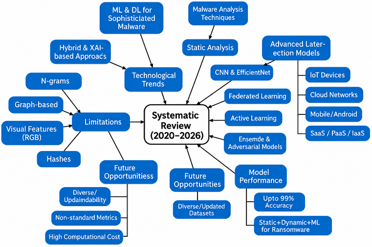
A common realization has been that the weakest link in the pipeline will bound the legitimacy of the results obtained. A sophisticated classifier cannot make up for the failure of a sandbox to trigger certain behavior, correct the mistakes made in reconstructing the graph, or filter out the labels from antivirus misclassification. Operational evaluations tend to cite considerations like cost of features, latency, abstention, analyst workload, and false positives less often than classification accuracy. Figure 1 is intended as a thematic map of the relationships among analysis methods, learning techniques, methodological limitations, and research directions. Table 1 summarizes these trade-offs.
Figure 1. Thematic relationship map of modern malware-detection research: analysis evidence, learning methods, methodological risks, and research directions
Table 1. Critical comparison of representative literature
|
Study |
Evidence/Model |
Main Contribution |
Critical Limitation |
|
Nataraj et al. [6] |
Binary images; texture features |
Established visual family classification without execution |
Visual similarity can be changed without changing behavior; no benign class in the original family task |
|
Raff et al. [8] |
Raw bytes; MalConv |
End-to-end learning from whole executables |
Input truncation, coarse pooling, and susceptibility to feasible byte manipulation |
|
Anderson et al. [12] |
EMBER PE features; LightGBM |
Large reproducible static benchmark and strong baseline |
Temporal and collection-specific bias; extracted features constrain alternative pipelines |
|
Pascanu et al. [15] |
System-event sequences; RNN |
Demonstrated value of sequential behavioral context |
Trace quality depends on activation, execution window, and sandbox realism |
|
Zhang et al. [41] |
API semantics + BiLSTM/TextRNN/attention |
Fused sequence order with action/resource semantics |
Complex preprocessing; attention is not automatically a causal explanation |
|
Ilić et al. [42] |
Full Cuckoo reports; RF |
Showed that evidence beyond API calls improves dynamic detection |
Single sandbox configuration; JSON representation can encode environment artifacts |
|
Alhashmi et al. [49] |
Static/dynamic APIs; XGBoost + ANN |
Used cross-view similarity as a hybrid signal |
Limited evidence on missing modalities, temporal drift, and external deployment |
|
Ling et al. [16] |
Hierarchical program graphs; GNN |
Preserved structural relations for robust Windows detection |
Graph extraction remains vulnerable to packing, disassembly errors, and indirect control flow |
|
Fang et al. [25] |
Federated Android detection |
Enabled collaborative learning without raw-sample exchange |
Client heterogeneity, poisoning, and privacy leakage remain deployment risks |
|
Walton et al. [29] |
LLM-assisted semantic categorization |
Connected malware artifacts to natural-language reasoning |
Reproducibility, hallucination, prompt sensitivity, and model-version drift |
Note: RNN: Recurrent Neural Network; GNN: Graph Neural Network; RF: Random Forest; LLM: Large Language Model; API: Application Programming Interface; JSON: JavaScript Object Notation; VM: Virtual Machine; URL: Uniform Resource Locator; ANN: Artificial Neural Network.
2.7 Research gaps
The main issues are of a methodological nature rather than resulting from the lack of new classifiers. The majority of experiments are still based on random splitting, overlapping classes, or one source document corpus, which helps learn corpus-specific patterns rather than any malicious activity. The robustness tests are too generic; real experiments should focus on functionality-preserving transformations like repacking, header modification, instruction replacement, function injection, and execution in analysis-aware environments.
A second gap concerns the evidence-acquisition process itself: many studies do not report execution coverage, empty traces, missing modalities, cross-sandbox transfer, or the end-to-end cost of collecting the evidence used by the classifier [13, 22, 43, 44].
The third group of weaknesses is related to trust and adaptation. The explanations are provided in the form of informative heat maps or feature importance rankings but are rarely analyzed in terms of accuracy, stability under semantically preserving transformations, or usefulness to analysts. Calibration, abstention, and alert workload also receive less attention than accuracy, even though they strongly influence whether a detector can operate at realistic malware prevalence. Continual and federated learning still face unresolved problems including poisoning, privacy leakage, catastrophic forgetting, delayed labels, client heterogeneity, and model-version control. Foundation-model assistance can provide useful summarization and semantic linking, but it should be retrieval-grounded, provenance-preserving, constrained in output, and subject to human approval [50, 61-63].
Table 2. Research gaps and recommended evaluation directions
|
Refs. |
Gap |
Current Weakness |
Recommended Direction |
Key Evidence to Report |
|
[9, 10, 13, 64] |
Temporal validity |
Random splits and outdated corpora |
Chronological, family-disjoint, and external validation |
Future-sample recall, open-set AUROC/AUPR, drift curves |
|
[13, 18, 37, 65] |
Adversarial robustness |
Abstract or single-attack testing |
Feasible, functionality-preserving, adaptive attack suites |
Robust recall, attack cost, functionality checks |
|
[16, 36, 53, 66] |
Semantic grounding |
Predictive features without behavioral meaning |
Map evidence to capabilities, actions, and causal chains |
Fidelity, semantic stability, analyst agreement |
|
[3, 42-44] |
Dynamic realism |
Single short sandbox run |
Multi-run, varied stimuli, cross-sandbox and bare-metal confirmation |
Execution coverage, empty-trace rate, cross-environment degradation |
|
[46, 49, 50, 67] |
Hybrid efficiency |
Accuracy reported without collection cost |
Cascaded, calibrated, missing-modality-aware fusion |
End-to-end latency, cost per sample, escalation rate |
|
[27, 36, 51, 52] |
Explainability |
Illustrative heat maps |
Stable, faithful, task-specific explanations |
Fidelity, consistency, investigation-time reduction |
|
[26, 58, 61, 68] |
Continual adaptation |
Static retraining schedules |
Drift monitoring, replay, regularization, active labeling |
Forgetting, adaptation delay, label budget |
|
[25, 57, 69, 70] |
Federated security |
Benign-client assumptions |
Robust aggregation, privacy accounting, poisoning tests |
Utility–privacy trade-off, attack success rate |
|
[29, 60, 71] |
LLM assistance |
Uncontrolled generation and opaque versions |
Retrieval grounding, constrained outputs, analyst approval |
Hallucination rate, provenance, reproducibility |
Note: LLM: Large Language Model; AUROC: Area Under the Receiver Operating Characteristic Curve; AUPR: Area Under the Precision–Recall Curve.
The main weakness is not a lack of new classifiers but the absence of a shared standard for judging evidence. Dataset provenance, semantic validity, temporal transfer, uncertainty, acquisition cost, and analyst impact are often reported separately even though they determine the same deployment claim. Table 2 summarizes the gaps and the evidence needed to make stronger claims. A convincing experiment should make clear what changed between training and testing, which inputs can be missing or manipulated, when the model is allowed to abstain, and what it costs to obtain the evidence used for a decision [4, 13, 23, 65, 72].
2.8 Contributions
From these gaps, five practical contributions follow:
(1) It groups the reviewed methods by the evidence they use and by the assumptions needed to obtain that evidence.
(2) It compares the methods on robustness, interpretability, computational burden, temporal validity, and deployment fit, rather than on accuracy alone.
(3) It shows how family overlaps, imbalance, missing modalities, sandbox configuration, and time-aware splitting can change what a reported score actually means.
(4) It integrates Transformers, graph models, explainable AI, federated learning, continual learning, and Large Language Model (LLM)-assisted analysis with the operational problems they are intended to address.
(5) It derives a research agenda centered on semantics-preserving robustness, calibrated uncertainty, cost-aware multimodal fusion, stable explanations, and reproducible time-aware benchmarks.
3.1 Malware fundamentals
3.1.1 Taxonomy and operational objectives
Classification schemes for malware are helpful in describing common goals, although modern specimens often combine features from different classes. A banking Trojan, for example, might include a rootkit, steal credentials, form a botnet, and then use ransomware. Using a single classification for the specimen is not sufficient, as it hides the complexity of the process. In detection studies, behavior-based classifications such as persistence, credential access, discovery, command-and-control, and impact are often a more robust target than specific families of vendors [1, 11, 73]. Table 3 describes common classes, typical evidence that they leave, and complexity of detection due to the behavior [1, 3, 4, 73].
Table 3. Major malware categories and detection implications
|
Refs. |
Category |
Primary Objective |
Common Evidence |
Principal Detection Challenge |
|
[1, 23, 24, 74] |
Virus |
Attaches to host files and replicates when the host executes |
File infection, modified entry point |
Polymorphism and legacy environments |
|
[1, 23, 24, 73-75] |
Worm |
Self-propagates across hosts |
Network exploitation, scanning, lateral movement |
Rapid spread and limited response window |
|
[1, 73, 76] |
Trojan/loader |
Disguises malicious capability or delivers payloads |
Social engineering, bundled software, compromised updates |
Benign appearance and staged execution |
|
[1, 73, 76, 77] |
Ransomware |
Encrypts or disrupts data; may exfiltrate before encryption |
Phishing, exploitation, remote services |
Early detection before destructive phase |
|
[1, 73, 77] |
Spyware/stealer |
Collects credentials, documents, or surveillance data |
Browser hooks, keylogging, form grabbing |
Low-noise, long-lived behavior |
|
[24, 73] |
Rootkit |
Conceals processes, files, or kernel modifications |
Driver or kernel manipulation |
Visibility below ordinary user-space tools |
|
[23, 73-76] |
Bot/botnet agent |
Provides remote control for coordinated activity |
C2 channels, DGA, peer-to-peer communication |
Traffic blending and infrastructure churn |
|
[23, 73-75, 77] |
Fileless malware |
Executes through memory and trusted interpreters |
PowerShell, WMI, macros, script engines |
Few persistent disk artifacts |
|
[73, 75-77] |
IoT malware |
Compromises resource-constrained connected devices |
Weak credentials, exposed services, firmware flaws |
Heterogeneous architectures and limited telemetry |
Family labels are to be considered noisy metadata, not the ground truth. Various vendors may assign different labels to one and the same lineage, merge different variants into one lineage, or change labels based on information about the campaign that emerges with time. These labeling noises need to be taken into account by the models of supervised learning, as they can cause classifier mistakes even if two samples share similar behavior. Research on malware families should address questions like aliasing, confidence threshold, and outliers, instead of assuming there is only one possible way of interpreting a family name [9-12].
Additionally, the notion of "sample" is itself unclear. Depending on the research, it can refer to a file hash, an unpacked payload, a module residing in memory, an Android package, a script, and the whole campaign. Equating those units can lead to mislabeling and wrong splitting into training and testing sets: several different droppers can drop the same payload, and a modular sample may change its behavior after obtaining other modules. Thus, studies should define clearly what they mean by file identity, lineage, behavior, and campaign, and specify what their task involves – binary detection, family classification, capabilities recognition, or campaign clustering [11, 13, 45].
3.1.2 Attack lifecycle and evidence generation
A typical malware attack will involve stages like delivery, exploitation, execution, persistence, privilege escalation, command and control, objective achievement, and adaptation. However, in practice, these attacks do not normally occur in a strictly sequential manner; a particular sample might backtrack to the discovery stage, gain another component, or just wait for an external signal before it begins its operation. Different artifacts are obtained through each phase, which are useful for detection purposes: static analysis for delivery, host-based detection for execution and persistence, network-based detection for command and control, and so on. Therefore, it is improbable for one detector alone to detect the whole attack. [3, 46, 73].
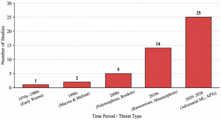
The importance of lifecycle reasoning is that it allows us to correlate each detection technique with the stage at which its evidence is generated. A pre-execution scanner can prevent a malicious file from doing any damage, but it cannot detect any credentials that have been acquired by an in-memory component. Conversely, a network detector can detect command-and-control activity only after execution has begun. Effective defense thus requires layering and evidence correlation, as we cannot assume that a single classifier is capable of seeing all of the stages. Figure 2 shows how the above operational process fits into the history of malware research, where increasing attention has been paid to adaptive and multi-stage attacks [1, 3, 73].
Figure 2. Evolution of malware topics from conventional threats to advanced and adversarial techniques
3.1.3 Evasion as a property of the detection problem
Evasion changes either the available evidence or the model’s interpretation of that evidence. Packing and encryption hide bytes from static inspection; anti- Virtual Machine (VM) checks reduce the behavior visible in a sandbox; process injection changes attribution; and adversarial edits target features learned by a classifier. The same technique can affect several stages. A packer may obscure static strings, delay unpacking, and expose only a benign stub during a short execution window. Robust systems therefore need evidence diversity and explicit tests against functionality-preserving transformations [4, 5, 18, 19].
A useful way to compare evasion is by the cost imposed on the attacker. Cosmetic metadata edits are inexpensive and can defeat brittle static features; repacking and code virtualization demand more effort but still preserve the malicious objective; environment-aware behavior requires the attacker to reason about execution context. Features that remain stable only under low-cost edits should not be treated as strong evidence.
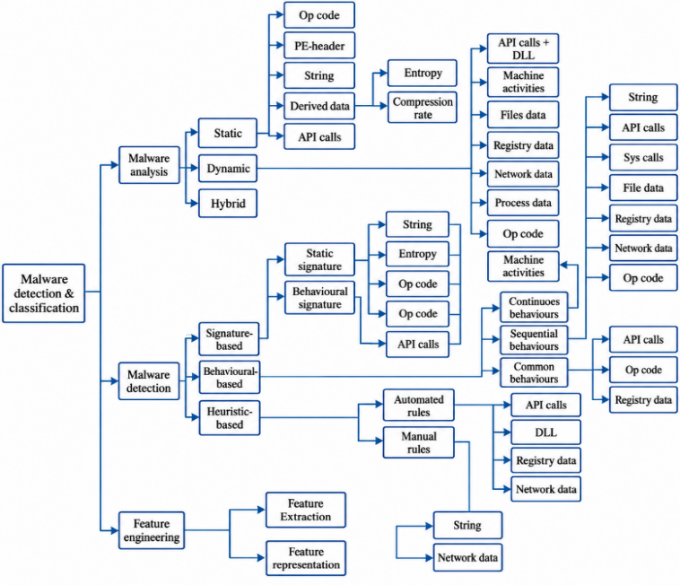
Figure 3 links the analysis mode to the evidence a detector can observe. That relationship should also guide robustness testing: a transformation is useful only if it is feasible under the stated threat model, not simply because it resembles a perturbation used in image classification [4, 18, 37, 65]. Table 4 takes the same view by matching evasion mechanisms to the evidence they disrupt and to practical countermeasures [4, 5, 37, 48].
Table 4. Malware evasion techniques and defensive implications
|
Refs. |
Technique |
Mechanism |
Most Affected Evidence |
Potential Countermeasure |
|
[4, 5, 48] |
Packing/encryption |
Conceals code until runtime |
Static bytes, strings, imports |
Unpacking, entropy/context analysis, memory inspection |
|
[5, 18, 37] |
Polymorphism |
Changes decryptor or signature across instances |
Signatures and byte n-grams |
Behavioral evidence, family-disjoint evaluation |
|
[5, 16, 33, 36] |
Metamorphism |
Rewrites equivalent instructions and control flow |
Opcodes, CFGs, image texture |
Semantic normalization and graph matching |
|
[3, 4, 43] |
Anti-debugging |
Detects breakpoints, timing, or debugger artifacts |
Manual and instrumented analysis |
Stealth instrumentation and multi-run analysis |
|
[3, 4, 43, 44] |
Anti-VM/sandbox |
Detects virtual hardware, low activity, or known tools |
Dynamic traces |
Realistic environments, interaction simulation, bare-metal confirmation |
|
[1, 42, 73] |
Process injection |
Runs inside a trusted process |
Process-name and parent-child heuristics |
Memory forensics and cross-process correlation |
|
[23, 73, 77] |
Fileless execution |
Uses scripts and trusted utilities in memory |
File scanning |
Script telemetry, AMSI-like inspection, memory and behavior analytics |
|
[18, 21, 37, 65] |
Adversarial feature manipulation |
Edits model-sensitive but nonfunctional regions |
ML/DL decision boundary |
Feasible-attack evaluation, robust features, adversarial training |
Note: ML: Machine Learning; DL: Deep Learning; CFG: Control-Flow Graph; VM: Virtual Machine.
3.2 Static malware analysis
Static analysis refers to the analysis of a file before execution. This analysis method is operationally favorable in the sense that hashes, headers, imports, strings, entropy, and some pieces of the code can be extracted quickly and reliably. The problem is that most of the static characteristics relate to how a file looks and are susceptible to modification by packing, modifying compilers, changing sections, and similar operations without modifying the behavior of the program [5, 12, 14, 30].
3.2.1 PE metadata, imports, strings, and entropy
Metadata for PE provides a brief summary of a binary on Windows, listing sections, their layout, the entry point, subsystem, imports, resources, their sizes, timestamps, and permissions. Initial work has shown that this metadata could be used to recognize new executables [30], while EMBER [12] expanded the representation by adding histograms of bytes, statistics on sections, imports, exports, and information about the file as such. The resulting combination of numerical, count, and categorical data becomes very suitable for use in tree-based models.
At the same time, convenience implies vulnerability. Many fields of metadata may be changed without impacting the operation of the program: fake timestamps, normalized names for sections, unused imports, imitation of normal values. While these features are useful, they are not supposed to be taken as reliable evidence.
Thus, the provenance of the features is as important as the features themselves. Multiple different feature vectors can be produced from the same binary depending on the version of the parser used, malformed headers, packed sections, or truncated vocabulary. A static analysis should be reproducible and list the parser and its version and report the number of extraction errors where possible. Otherwise, some part of the model may reflect the assumptions of a specific parser instead of malware features generalized over the contexts. This problem is similar to the first attempts of formal specification of malicious behavior [78].
Static parsers can also recover Uniform Resource Locators (URLs), registry keys, command strings, cryptographic calls, process-manipulation APIs, and anti-analysis indicators. Such artifacts are cheap to inspect and often meaningful to analysts, but they are easy to hide through encryption, runtime loading, or small loader stubs. Entropy may suggest packing or encryption, yet legitimate installers and multimedia files can also have high entropy. No single artifact should therefore carry much evidential weight; the strongest static claims combine several independent signals and document how unresolved or missing features were treated [2, 12, 14, 32, 78].
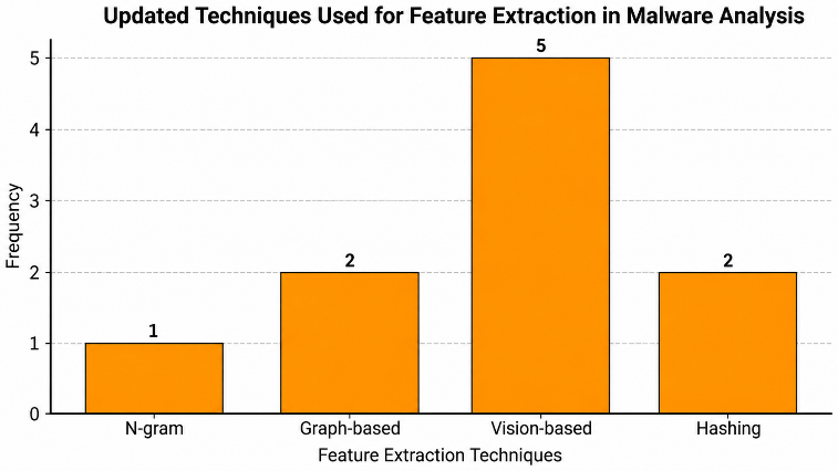
The static features can be sorted by the cost of manipulating them. File hashes and exact byte signatures are highly discriminative but may be fragile; header fields and imports are inexpensive to edit but carry less semantic meaning; opcode and graph representations are more semantic but require reliable disassembly; and data-flow properties are difficult to modify without affecting functionality, yet they are typically much more costly to recover. This hierarchy indicates a realistic approach to designing inexpensive, editable indicators for quick triage and more expensive semantic analysis for more ambiguous or critical files. Figure 4 summarizes the range of extraction techniques commonly used to implement this progression [5, 30, 31, 78].
3.2.2 Byte, opcode, and graph representations
Byte n-grams capture local patterns and do not disassemble, but they have a rapidly expanding vocabulary that can be affected by compiler and packer artifacts [31]. Opcode sequences eliminate some of the operand jargon and get closer to the semantics of the instruction, but disassembly is hard in packed, obfuscated, or self-modifying binaries. Control-flow and call graphs capture the relationships between blocks and functions and are appealing to GNNs [16, 33-36]. Cost is pushed upstream: an incorrect graph can lead to a sophisticated model reasoning over an incorrect program representation with confidence.
There is a second source of uncertainty, which is often masked in final accuracy numbers, that occurs when constructing graphs. It is possible to have incomplete or incorrect graphs because of indirect calls, exception-driven control flow, stripped symbols, overlapping instructions, and self-modifying code. Canonicalization can eliminate some differences on the surface, but it can also eliminate some rare behavior that differentiates a malicious branch. The results of graph-based studies should therefore include an indication of which nodes were successfully disassembled, the distribution of the size of the graph, any isolated nodes, any edges that were not resolved, and the impact of failures in the extraction. If the issue is not accounted for, an apparent gain from a GNN could be a consequence of a cleaner subset of samples, instead of improved reasoning about program structure [16, 33-35].
3.2.3 Raw-byte and image-based learning
Raw-byte learning and malware images reduce handcrafted feature design. MalConv [8] processes byte embeddings directly, while image approaches reshape bytes or derived statistics into two-dimensional patterns [6, 7, 14]. Image conversion is efficient and benefits from mature CNN architectures, but spatial adjacency in an image is imposed by the encoding rather than by program execution. A model may detect family-specific texture, padding, or packer style rather than malicious behavior. External validation on temporally separated and differently packed samples is therefore more informative than additional accuracy on the same image benchmark.
Table 5. Comparison of static feature representations
|
Refs. |
Representation |
Typical Features |
Strength |
Limitation |
|
[12, 30, 32] |
PE metadata |
Header fields, sections, imports, resources |
Fast, compact, interpretable |
Fields are editable and may encode collection artifacts |
|
[2, 12, 14] |
Strings/imports |
Text, URLs, paths, API names |
Direct analyst meaning; low cost |
Encrypted strings and dynamic resolution hide evidence |
|
[14, 31] |
Byte n-grams |
Local raw-byte subsequences |
No disassembly; strong local signatures |
Very high dimension; sensitive to insertion and packing |
|
[8, 18, 37] |
Raw bytes |
Learned embeddings from executable stream |
End-to-end representation learning |
Truncation, pooling loss, feasible adversarial edits |
|
[5, 33] |
Opcodes |
Instruction sequences or frequencies |
Closer to code semantics than bytes |
Disassembly errors; operand and control-flow context lost |
|
[16, 33, 36] |
CFG/call graph |
Blocks/functions and their relations |
Preserves structure and supports GNNs |
Graph recovery is costly and fragile under obfuscation |
|
[6, 7, 79] |
Malware image |
2D byte/entropy/color encoding |
Scalable; leverages vision models |
Image geometry is artificial; texture may reflect packers |
Note: PE: Portable Executable; GNN: Graph Neural Network; CFG: Control-Flow Graph; API: Application Programming Interface; URL: Uniform Resource Locator.
Table 6. Representative static-analysis studies
|
Study |
Input |
Model |
Contribution |
Primary Limitation |
|
Schultz et al. [30] |
Metadata, strings, byte sequences |
Data-mining classifiers |
Established learning-based detection of new executables |
Small early corpus and features tied to the period |
|
Saxe and Berlin [14] |
Bytes, entropy, imports, metadata |
DNN |
Integrated heterogeneous static evidence |
Handcrafted extraction and uncertain robustness to feature manipulation |
|
Raff et al. [8] |
Raw executable bytes |
MalConv |
End-to-end large-file classification |
Truncation, coarse pooling, adversarial append attacks |
|
Anderson and Roth [12] |
Engineered PE features |
LightGBM baseline |
Reproducible, large-scale benchmark |
Temporal bias and fixed extracted representation |
|
Yan et al. [33] |
Control-flow graphs |
Deep GCN |
Captured structural program relations |
Depends on accurate CFG construction |
|
Ling et al. [16] |
Hierarchical graphs |
Hierarchical GNN |
Improved structural robustness |
Extraction cost and limited evidence under packing |
|
Basak et al. [79] |
Binary-derived images |
DRIN |
Lightweight involution/residual feature learning |
Image semantics and external robustness remain uncertain |
Note: PE: Portable Executable; GNN: Graph Neural Network; URL: Uniform Resource; DNN: Deep Neural Network.
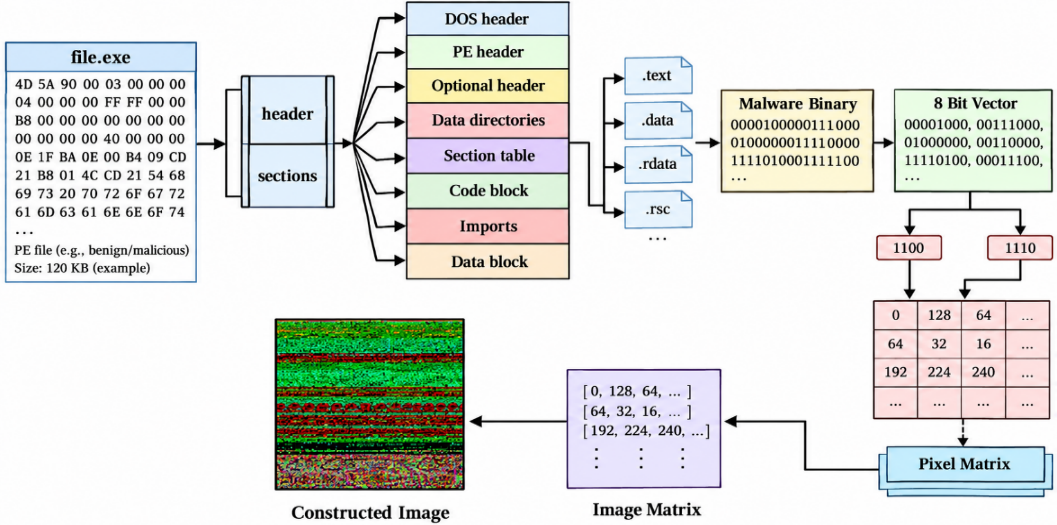
The most informative validation for raw-byte and image models is not another random split of the same corpus. It is performance under a changed packer, compiler, collection period, or benign-software source. Packer-stratified tests can reveal whether the model recognizes malicious content or merely a protection tool; salting and section-injection tests expose sensitivity to non-executed regions; and family-disjoint evaluation measures whether the learned representation extends beyond near-duplicate variants. Many visual pipelines convert the binary to an image, as shown in Figure 5, and it is important to remember that the geometry obtained is one of modeling and not a native property of program execution [6-8, 12].
Tables 5 and 6 are different in that Table 5 compares the features of the major static representations, while Table 6 indicates how these representations were applied in selected studies and where the major methodological limitations [5, 12, 14, 79].
Static analysis is most convincing as a quick first-pass filter. It is not very suitable for triage or risk scoring, and it can't define full behavior on its own. Evaluation must then encompass various packers and friendly vendors, timeouts, and edits that preserve functionality. Dynamic/hybrid analysis is the next step up from a static analysis when a sample is still uncertain or high impact, rather than making a confident static label.
Combined, Tables 5 and 6 illustrate why static features are still of operational value while also requiring clear extraction, time-aware testing, and protection from realistic representation changes [5, 12, 14, 79].
3.3 Dynamic malware analysis
Dynamic analysis observes a sample while it runs in an instrumented environment. The trace may include API calls, spawned processes, file and registry changes, memory activity, persistence actions, Domain Name System (DNS) traffic, sockets, and downloaded content. These observations are behaviorally richer than file metadata, but they are not complete: operating-system version, privileges, user activity, network access, execution duration, and sandbox artifacts all influence what appears in the trace [3, 15, 43, 44].
3.3.1 Sandboxing and behavioral telemetry
CWSandbox [43], Ether [44], and later open platforms such as Cuckoo illustrate different trade-offs between observability and transparency. Virtualized sandboxes are scalable and resettable, but they can be fingerprinted. Bare-metal analysis reduces some virtualization artifacts, yet it is more expensive to orchestrate and restore. No environment is perfectly transparent. A practical design uses multiple runs, varied stimuli, and explicit reporting of non-executing samples rather than silently discarding them.
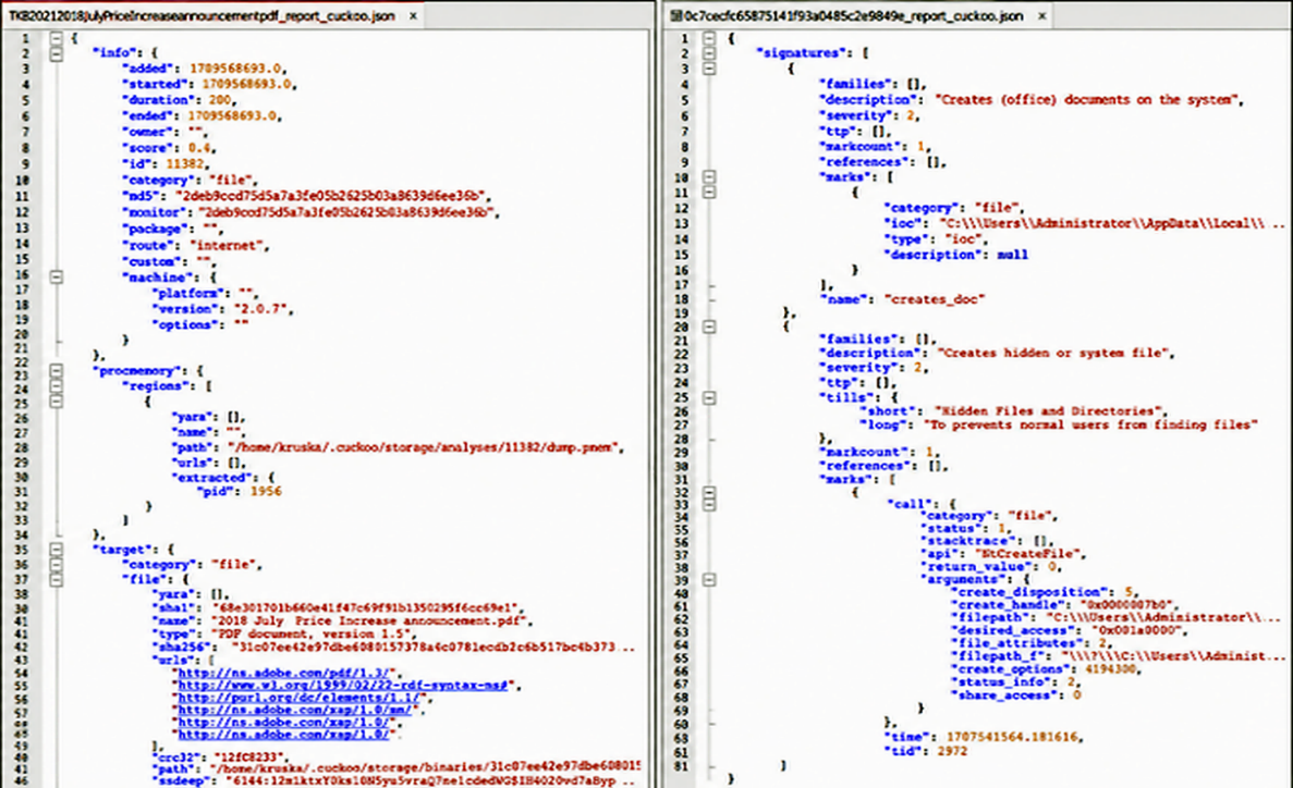
Behavioral coverage is not assumed and should be quantified. Some useful metrics are the percentage of samples that successfully start; the number of unique processes and actions seen; the percentage of samples with network activity and the percentage with persistence; and the difference between evidence seen in multiple runs. This sort of reporting differentiates a model that learns from rich behavior from one that is judged based on empty, truncated, or environment-specific reporting. It also brings the latency–coverage trade-off to the practitioners. Previous automated behavior-clustering studies also demonstrated that dynamic labels and clusters are only as valid as the actions that are triggered by the execution environment [45]. Figure 6 shows the amount of information contained in real Cuckoo reports and how this information can be lost when a report is limited to API names [42].
Repeated execution is particularly critical for nondeterministic or trigger-dependent malware. The different actions of users, the local environment, the age of the system, the content of the documents, the permissions granted to the users, and the response of the network can reveal branches that were not identified in a single run. The traces that result should not just be strung together without provenance; analysts should be able to determine which behavior was consistently present and which was dependent upon a specific stimulus. A detailed look at the variety and depth of full sandbox reports. Figure 6 provides a concrete view of the richness and heterogeneity of full sandbox reports, illustrating why dynamic analysis is an experimental measurement process rather than a deterministic file parser [3, 4, 42].
3.3.2 Application Programming Interface sequences, semantics, and behavioral graphs
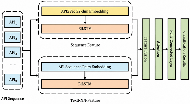
Popular options are API calls, which are easy to extract and naturally map to sequence models. Frequency vectors are brief, without order. RNNs and GRUs maintain order but may have difficulty with extremely long traces. CNNs are used to capture local motifs and attention; Transformers are used to capture wider dependencies, and behavioral graphs represent causal or temporal relations. The representation should also preserve arguments and context, if possible. CreateFile and WriteFile are not in themselves negative things; meaning is given by the path, calling, process ancestry, timing, and subsequent network behavior. A related lesson from Android is that it has seen some success with API-level features and Markov abstractions, but the transfer will rely on the evolution of the platform, the choice of abstraction, and the stability of the platform vocabulary [55, 56]. Figure 7 shows one open-access architecture that attempts to preserve both sequence order and semantic information rather than treating calls as isolated tokens [41].
Mal-ASSF [41] shows semantic enrichment by associating the type of action and the resource in the name of an API. Ilić et al. [42] demonstrate the incompleteness of API-only pipelines: in their context, complete sandbox reports better performance than call sequences. The important takeaway is not that one thing always prevails, but that behavior is multi-channel. A detector should be able to maintain provenance for an analyst to determine if evidence is from a parent process, injected thread, child process, or network component.
The order of the events is also insufficient if they are coming from multiple processes or threads. Even if both invoke similar APIs, the process ancestry, call arguments, return values, object identifiers, and time gaps help distinguish a benign installer from a malicious injector. These relations can be represented by behavioral graphs and event-correlation models, but these require more storage and more preprocessing and are sensitive to instrumentation. Figure 7 illustrates the use of both sequence and semantic evidence; its overall message is that no API name is very informative when taken alone, but when considered together with its operation type, target resource, and surrounding context, it becomes more informative [15, 38-40].
No sequence model can infer an action that never appears in the trace. Dynamic studies should therefore report how many samples executed successfully, how long they ran, what stimulation was used, which environmental fingerprints were present, and how many traces were empty or incomplete. Cross-sandbox testing is especially useful because the instrumentation itself may become an unintended label. Tables 7 and 8 summarize these evidence sources and representative dynamic studies [3, 42, 43, 45].
Table 7. Dynamic evidence sources and limitations
|
Refs. |
Evidence |
Examples |
Analytical Value |
Main Limitation |
|
[15, 38, 41, 42] |
API calls |
Names, counts, order, arguments |
Compact behavioral vocabulary |
Call injection, truncation, missing context |
|
[42-45] |
Process telemetry |
Creation, injection, ancestry, privileges |
Reveals staging and trusted-process abuse |
Attribution becomes difficult under injection |
|
[3, 42, 43] |
File/registry |
Create, modify, delete, persistence keys |
Interpretable evidence of installation and impact |
Benign installers can look similar |
|
[3, 42, 45] |
Network activity |
DNS, IPs, TLS metadata, timing, payloads |
Exposes C2 and exfiltration |
Encryption, infrastructure churn, offline payloads |
|
[3, 42, 44] |
Memory events |
Allocations, permissions, unpacked code |
Can reveal fileless and unpacked payloads |
High collection and storage cost |
|
[42, 43, 80] |
Full sandbox report |
Cross-channel JSON or event graph |
Preserves complementary evidence |
Environment-specific artifacts and high dimensionality |
Note: API: Application Programming Interface; JSON: JavaScript Object Notation.
Table 8. Representative dynamic-analysis studies
|
Study |
Evidence |
Model |
Contribution |
Primary Limitation |
|
Pascanu et al. [15] |
System-event sequences |
RNN |
Captured dependencies beyond event counts |
Long traces and payload non-activation |
|
Kolosnjaji et al. [38] |
API/system-call sequences |
CNN + RNN |
Combined local motifs and temporal order |
Sandbox-specific traces and limited call semantics |
|
Huang and Stokes [39] |
Behavioral sequences |
Multitask neural network |
Shared detection and family-learning signals |
Transfer across environments not established |
|
Rhode et al. [81] |
Early runtime behavior |
RNN |
Investigated early-stage prediction |
Latency–evidence trade-off and dataset specificity |
|
Zhang et al. [41] |
API sequences + semantics |
BiLSTM/TextRNN/attention |
Added action/resource semantics |
Preprocessing complexity and attention instability |
|
Ilić et al. [42] |
Full Cuckoo reports |
RF |
Evidence beyond APIs improved results |
Single analysis environment and representation artifacts |
|
Syeda and Asghar [80] |
API counts and categories |
Six classical ML models |
Feature scoring and behavioral categorization |
Modest executed sample count and no cross-sandbox validation |
Note: RNN: Recurrent Neural Network; CNN: Convolutional Neural Network; API: Application Programming Interface; ML: Machine Learning; RF: Random Forest.
3.4 Hybrid malware analysis
Hybrid analysis combines what can be learned before execution with what becomes visible at runtime. Static evidence is inexpensive and complete for the file that is present; dynamic evidence is richer semantically but incomplete and costly to collect. Fusion may occur at the feature, representation, score, or decision level. The practical advantage comes from preserving which modality produced each piece of evidence and from handling missing or conflicting views explicitly [28, 46, 47, 49].
3.4.1 Fusion strategies and operational cost
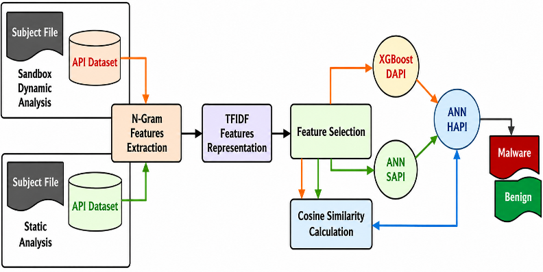
Early fusion concatenates static and dynamic features before classification. Although straightforward, dimensional imbalance and redundancy can cause one modality to dominate the decision. Intermediate fusion: Learn the encoders separately and fuse the latent representations. This aids modality-specific processing, and failure to attribute is more difficult. Late fusion is the combination of calibrated scores or decisions, and it is simpler to audit, but it might fail to capture cross-modal interactions. A cascaded design (static triage plus dynamic escalation) can provide the optimal operational balance since only those files that are in limbo or high risk are subjected to sandbox cost. As a concrete example of score- and similarity-based hybridization, the static and dynamic API evidence can be combined without assuming that the two views are the same [49].
Failure cases should be incorporated into hybrid evaluation, which can otherwise obscure them. A sample may have a valid static view but no dynamic trace, or these may be quite different and produce sharply conflicting scores. The system should indicate whether it imputes the missing view, abstains from making a decision, or escalates the sample, along with an explanation of how each policy affects latency and the rate of false positives. This approach is more informative than assessing only samples for which all of the analysis components were successful. This evaluation should account for modality ablation, deliberate corruption of the views, and calibration experiments to prevent an apparent gain due to one predominant branch or due to accidental matchings between correlated features [28, 46-49].
Disagreement between static and dynamic views can itself be informative. An imported networking function that never executes may indicate an unused branch, sandbox evasion, or insufficient stimulation. A function observed at runtime but absent from the import table may instead point to late binding or obfuscation. HAPI-MDM (Figure 8) illustrates this relational use of static and dynamic API evidence. Future fusion methods should report whether cross-view consistency improves robustness or merely adds correlated features [46, 48, 49].
Table 9 places static, dynamic, and hybrid analysis side by side, focusing on how each strategy acquires evidence, where it is strongest, and what limits its use in practice.
For hybrid systems, acquisition policy matters as much as classifier accuracy. Running every file in a sandbox may improve coverage but is difficult to scale; a calibrated cascade can reserve expensive analysis for uncertain or high-impact samples. Escalation rate, mean and tail latency, and risk reduction per unit of compute are therefore more informative than a single fused accuracy score. These systems should be judged with latency, coverage, and calibration in addition to predictive performance [28, 46, 49, 50].
Table 9. Static, dynamic, and hybrid analysis strategies
|
Refs. |
Strategy |
Strength |
Weakness |
Best-Fit Use |
|
[5, 8, 12, 13] |
Static only |
Low feature cost; deterministic and scalable |
Packing, metadata manipulation, limited runtime semantics |
Gateway scanning and large-scale triage |
|
[3, 15, 42, 43] |
Dynamic only |
Behavioral context; resilient to many static obfuscations |
Sandbox evasion, latency, incomplete execution |
Deep analysis of suspicious samples |
|
[46-49] |
Early hybrid fusion |
Captures cross-modal interactions in one model |
High dimensionality, redundancy, missing-modality sensitivity |
Offline research and controlled pipelines |
|
[28, 49, 53] |
Intermediate multimodal fusion |
Separate encoders learn modality-specific representations |
Opaque modality contribution and training complexity |
Rich multimodal classification |
|
[46, 49, 50] |
Late/score fusion |
Auditable, modular, tolerant of model replacement |
Requires calibrated scores; fewer low-level interactions |
Operational SOC pipelines |
|
[47, 50, 67] |
Cascaded analysis |
Balances throughput and depth |
Errors in first-stage triage can block escalation |
Enterprise and cloud-scale deployment |
Hybrid performance is meaningful only when the full collection cost is reported. Useful reporting includes sandbox throughput, failed executions, feature-storage overhead, behavior under missing modalities, and latency at each stage. A small accuracy gain is hard to justify if it multiplies analysis time, whereas a calibrated cascade may reduce cost without sacrificing risk control. Table 9 therefore compares early, intermediate, late, and cascaded fusion not only by analytical strength but also by deployment burden [28, 46, 47, 49].
4.1 Classical machine learning models
Classical ML remains important because many malware features are sparse, heterogeneous, or tabular. RFs and boosted trees handle nonlinear interactions well; SVMs remain effective in high-dimensional sparse spaces; logistic regression provides a transparent baseline; and nearest-neighbor methods can support similarity search. These models are generally cheaper to train and easier to inspect than deep networks, although their performance depends more heavily on the stability of engineered features [12, 30, 31, 80].
4.1.1 Trees, margins, neighborhoods, and ensembles
RFs [82] provide strong baselines for PE metadata and dynamic-report vectors, although their probabilities may require calibration and high-cardinality artifacts can be memorized. SVMs [83] work well with sparse n-grams and API indicators but become expensive with some kernels at scale. XGBoost [84] and LightGBM [85] are effective on heterogeneous static features because they model nonlinear interactions efficiently. None is immune to drift: a split on a compiler timestamp or section count can age just as quickly as a neural feature.
Nearest-neighbor retrieval is intuitive for family similarity, but distance becomes less informative in very high-dimensional spaces and the reference set can be expensive to store and search. Decision trees (DT) [86] are easy to inspect, yet a single tree is unstable and can overfit. Ensembles reduce variance only when their components add genuine diversity; several models trained on the same leaked split can simply reproduce the same shortcut.
The feature space should guide model choice. Sparse n-grams often suit linear margins, mixed PE fields often favor boosted trees, and similarity search may require a purpose-built metric rather than ordinary nearest neighbors. Hyperparameter tuning belongs entirely inside the training period in temporal experiments; using later samples for tuning leaks future information even when their labels are hidden. Feature importance also needs context, since a timestamp, signer, or section name can be a collection artifact rather than a malicious capability [10, 12, 13, 82]. Figure 9 summarizes the main classical model families discussed in this review and the operational roles for which they are commonly suited.
Table 10. Classical machine-learning algorithms for malware detection
|
Refs. |
Algorithm |
Typical Input |
Advantages |
Limitations |
|
[12, 74, 76] |
Logistic regression |
Sparse PE/API indicators |
Fast, interpretable baseline; often well calibrated |
Linear boundary unless features encode interactions |
|
[74, 75, 86] |
Decision tree |
Mixed tabular features |
Readable rules and low inference cost |
High variance and shortcut learning |
|
[12, 74, 82] |
RF |
PE metadata, sandbox report vectors |
Strong nonlinear baseline; handles mixed features |
Large ensembles and weak extrapolation under drift |
|
[31, 74, 83] |
SVM |
Byte/opcode n-grams, sparse permissions |
Effective in high-dimensional spaces |
Scaling and probability calibration |
|
[31, 74] |
KNN |
Image or embedding similarity |
Simple family retrieval and local decisions |
Expensive inference; distance degradation in high dimensions |
|
[12, 64, 84, 85] |
XGBoost/LightGBM |
Engineered PE and behavior features |
High accuracy and efficient tabular learning |
Sensitive to dataset artifacts and changing feature distributions |
|
[74, 76, 77] |
Stacking/voting |
Multiple classifiers or modalities |
Can combine complementary errors |
Benefits vanish when base models share the same bias |
Note: SVM: Support Vector Machine; KNN = K-Nearest Neighbors; PE: Portable Executable; API: Application Programming Interface; RF: Random Forest.
When selecting a model, the probability quality, maintenance burden, as well as predictive accuracy should be taken into account. When it can be transferred across time, is cheap to retrain, and provides helpful feature diagnostics, an RF or boosted tree may be the more suitable operational choice. A bigger model is warranted if it shows interactions that stay consistent on subsequent or external data. It is important to note that calibration should be checked after temporal shift, as ranking performance may be satisfactory even if probability estimates are overconfident [22, 50, 82, 84].
Threshold analysis is also necessary for production use, not default class labels. The number of alerts may be excessive, even when the model is not of lower quality, if the probabilities are miscalibrated at realistic prevalence. In addition to feature extraction time and memory requirements, post-hoc calibration, cost-sensitive thresholds and an abstention region should be taken into account [50, 87, 88]. Good classical models must meet minimum standards. This is not a bad result because a boosted tree is superior to a much larger neural network for the same time-aware split. If there is additional complexity that does not add to transfer, robustness, calibrated uncertainty, or analyst value, then it is not worth it. Table 10 presents a summary of the appropriate applications and major failure modes of typical classical algorithms [12, 30, 42, 82].
4.2 Deep learning models
4.2.1 CNNs and visual malware representations
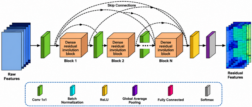
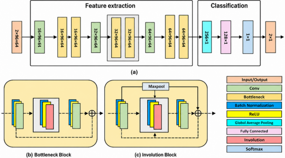
CNNs learn local patterns in byte streams, entropy maps, opcode matrices, or malware images [6-8, 14]. Their parameter sharing is well suited to repeated motifs, and transfer learning can reduce data requirements. However, the visual encoding defines what locality means. Adjacent pixels may represent neighboring bytes rather than related instructions, and resizing can remove or distort file structure. High benchmark accuracy should therefore be accompanied by packed-sample, external-dataset, and family-disjoint tests. Figures 10 and 11 reproduce the open-access Dynamic Residual Involution Network (DRIN) overview and architecture, providing a concrete example of how modern visual malware models combine residual pathways, multi-scale processing, and involution-style operators [79]. Figures 10 and 11 provide the corresponding open-access model overview and detailed architecture, respectively.
4.2.2 Recurrent networks and transformer models
LSTM [89] and GRU-based sequence models used in malware analysis [40] are natural choices for API and system-call sequences because they preserve event order and mitigate the vanishing-gradient problem. They remain effective for moderately long traces, but sequential computation and limited memory make very long histories difficult. BERT-like contextual encoders [90] provide bidirectional representations, while Transformers [91] use attention to model more distant relations.
Vision Transformers build on this concept and learn long-range relationships between image patches to represent image-based malware. The benefit of the standard Vision Transformer and hierarchical Swin Transformer in malware analysis will rely on whether the binary-to-image encoding retains meaningful global relations [92, 93], as the structure of malware is different from that of natural images. Care should thus be taken to control for the following factors in comparative studies: pretraining, resolution, parameter count, and augmentation; otherwise, an improvement due to attention may be due to a larger model or more favorable training recipe [53, 79, 92, 93].
Explicit analysis of long-trace handling is warranted due to truncation, padding, and sampling, which determine the behavior that reaches the model. Early activity can be favored by only keeping the first calls, while the last calls may be missed, and uniform subsampling can kill rare but crucial calls. There are alternatives including hierarchical encoders, chunk-level attention, and event-type-aware compression, but each comes with assumptions that need to be evaluated via ablation. Pretraining on large unlabeled traces is encouraging as long as the pretraining corpus and the test period are separated in order to prevent temporal contamination [15, 38-40].
4.2.3 Graph Neural Networks, explainability, and multimodal models
GNNs operate on CFGs, call graphs, and interaction graphs [16, 33-36]. They can learn from relational structure that flat sequences lose, but they inherit every error in graph construction. Explanation methods such as Grad-CAM [51], LIME [52], SHAP [94], and LEMNA [66] help expose influential features or regions. None should be treated as proof of malicious intent. Explanations should be stress-tested for stability, fidelity, and sensitivity to semantics-preserving transformations, and they should connect model evidence to analyst-relevant behavior. Figure 12 shows an open-access hybrid CNN-Transformer design with Grad-CAM explanations, while Table 11 compares the evidence, strengths, and limitations of the principal deep-learning families used in malware research [53, 92, 93, 95].
Table 11. Deep-learning architectures used in malware detection
|
Refs. |
Architecture |
Typical Input |
Strength |
Principal Limitation |
|
[8, 14, 32] |
1D CNN/raw-byte model |
Raw bytes or opcode stream |
Fast local feature learning |
Limited global context; feasible byte manipulation |
|
[6, 7, 79] |
2D CNN |
Malware images/matrices |
Mature vision backbones and transfer learning |
Encoding-dependent semantics and benchmark bias |
|
[15, 38, 40, 81] |
LSTM/GRU |
API, opcode, or audit sequences |
Temporal order and variable-length modeling |
Slow sequential processing; long-trace forgetting |
|
[17, 53, 90, 91] |
Transformer/BERT |
Tokenized API or opcode sequences |
Long-range context and parallel training |
Memory cost, data demand, truncation, unstable interpretations |
|
[16, 33, 36] |
GNN |
CFG, call graph, behavior graph |
Relational and hierarchical structure |
Graph recovery cost and sensitivity to obfuscation |
|
[77, 79, 96] |
Autoencoder/self-supervision |
Unlabeled bytes, images, or telemetry |
Reduces label dependence; anomaly representation |
Reconstruction may prioritize benign variance over malicious semantics |
|
[28, 49, 53] |
Hybrid/multimodal network |
Static + dynamic or CNN + Transformer |
Complementary representations |
Fusion opacity, missing modalities, high deployment cost |
|
[29, 60, 71] |
LLM-assisted analysis |
Reports, APIs, threat intelligence, decompiled text |
Semantic summarization and analyst support |
Hallucination, prompt sensitivity, privacy, reproducibility |
Note: GNN: Graph Neural Network; API: Application Programming Interface; CNN: Convolutional Neural Network.
Recent visual classifiers increasingly combine convolutional locality with Transformer context. Alshomrani et al. [53], for example, fuse ConvNeXt [95] and Swin Transformer [93] features and use Grad-CAM to inspect predictions. The architecture is representative of a wider move toward multi-backbone learning. What matters scientifically is whether the branches contribute complementary evidence on unseen data and whether the extra complexity remains acceptable at deployment, not simply whether fusion lifts validation accuracy.
Multimodal DL should be evaluated with modality dropout and branch-specific ablation. If performance remains unchanged when a dynamic or graph branch is removed, the advertised fusion may be largely decorative. Conversely, a model that collapses when one view is missing is unsuitable for real pipelines where extraction routinely fails. Robust multimodal systems need confidence-aware fusion, missing-view training, and explanations that identify which source changed the verdict. Figure 12 illustrates a modern CNN–Transformer design, while the evaluation requirement extends beyond visual accuracy to branch contribution, calibration, and computational cost [53, 79, 93, 95].
DL is most valuable when it learns a representation that remains useful across time, families, and environments. A larger architecture is not a substitute for honest evaluation. External validation, uncertainty calibration, ablation of each modality, and robustness to feasible edits should be standard requirements before a model is described as suitable for deployment. The architectures summarized in Table 11 should therefore be interpreted as alternative evidence-processing mechanisms, not as a ranking independent of dataset design, tokenization, graph recovery, or deployment cost [16, 33, 34, 36].
5.1 Public malware datasets
Dataset choice often determines the apparent difficulty of a malware problem. Family-classification corpora, binary detection corpora, Android application sets, dynamic traces, and image datasets support different claims. A model evaluated only on malware families cannot establish benign-versus-malicious detection. A dataset collected in one period cannot establish future robustness. Public datasets improve reproducibility, but many contain label noise, family imbalance, duplicates, missing timestamps, or features extracted by an obsolete toolchain [9, 12, 42, 96].
Public benchmark development has also expanded from competition-oriented datasets such as the Microsoft Malware Classification Challenge (BIG 2015) [97] to substantially larger resources such as MalNet [98], which provides image- and graph-based representations at scale. Benign examples deserve the same curation discipline as malware. If the benign set comes from one operating-system installation or one software repository, a classifier may separate vendors, signers, or build practices instead of malicious behavior. Antivirus-consensus labels introduce another issue: the results of scans may vary when it comes to borderline cases. It is important for benchmark designers to acknowledge this level of ambiguity, avoid rejecting tricky cases once the results are out, and indicate whether the labels were fixed at the point of collection or later revised. In terms of Android, several issues include the era of Drebin, consensus labels used by AndroZoo, and changes made to the platform that affect DroidAPIMiner and MaMaDroid [54-56, 99].
It is necessary to describe the lineage of datasets in question at the file and campaign levels. Hash deduplication filters out exact duplicates but does not eliminate recompiled or slightly altered samples; thus, family leakage can still happen. The mitigation measures include similarity-based deduplication, timestamp data, signer info, and lineage-aware grouping. Provenance of the labels is also essential: manual labelling, labelling by campaigns, and antivirus consensus make different scientific claims. Noisy binary labels are sufficient for preliminary analysis but not enough for detailed family classification [11-13, 22].
Table 12. Frequently used public malware datasets
|
Dataset |
Platform/Modality |
Approximate Scale |
Best Use and Main Caveat |
|
Malimg [6] |
Windows malware images |
9,339/25 families |
Image family classification; no original benign class; older families |
|
BIG 2015 [97] |
Windows bytes and assembly |
10,868 labeled/9 families |
Large benchmark, but competition-era families and no benign class |
|
EMBER [12] |
Windows Portable Executable (PE) features |
≈1.1M files |
Reproducible binary detection; fixed engineered features and dated collection |
|
SOREL-20M [9] |
Windows PE features/metadata |
≈20M files |
Scale and auxiliary tags; substantial storage and label-source dependence |
|
BODMAS [10] |
Windows PE features/binaries |
134,435 files; 581 malware families |
Timestamps support drift studies; collection still limited to one period |
|
MOTIF [11] |
Windows malware with expert family labels |
3,095/454 families |
High-quality family ground truth; no benign class and small per-family counts |
|
EMBER2024 [64] |
Holistic Windows benchmark |
Large modern corpus |
Designed for broader evaluation; recent and still establishing baselines |
|
MalNet [98] |
Malware images/graphs |
≈1.2M samples; 47 types |
Scale and multiple modalities; taxonomy and duplicate control require care |
|
Drebin [54] |
Android static features |
5,560 malware/179 families |
Classic reproducible benchmark; Android ecosystem is now dated |
|
AndroZoo [99] |
Android Android Package Kit (APK) repository |
Millions of apps |
Scale and timestamps; labels depend on external antivirus consensus |
|
Virus-MNIST [96] |
PE thumbnails |
≈50,000/10 classes |
Accessible image benchmark; first-1,024-byte view is highly reductive |
|
MaleVis [100] |
RGB malware/benign images |
14,226/26 classes |
Balanced training images; visual encoding and family age limit inference |
|
Ilić et al. [42] |
Dynamic Windows reports |
22,200 benign/malicious reports |
Rich behavior beyond APIs; tied to one sandbox configuration |
Dataset governance should include a written version policy. Labels may change as vendors acquire new intelligence, family aliases may be merged, and legal restrictions may alter sample availability. A benchmark should therefore publish immutable split manifests, hashes or stable identifiers, feature-extractor versions, label timestamps, and a changelog that distinguishes corrected metadata from newly collected samples. EMBER2024 is a useful step because it broadens file-format and task coverage, but its long-term value will depend on transparent versioning and independent reproduction of its evaluation protocols [9-12].
Platform coverage is itself a dataset-design constraint. Windows PE has the richest set of reusable benchmarks in the literature reviewed here, whereas Android research is supported by corpora such as Drebin and large repositories such as AndroZoo [54, 99]. IoT studies more often rely on device- or network-specific telemetry and may be evaluated within federated or incremental-learning settings [57, 58]. Comparable public corpora for cloud-native workloads, containers, scripts, and memory-resident attacks are less standardized. Accordingly, cross-platform conclusions in this review concern transferable evaluation principles—provenance, temporal separation, uncertainty, acquisition cost, and robustness—rather than an assumption that the same features or benchmark maturity apply uniformly to every platform.
A defensible protocol should record stable identifiers, deduplication rules, collection dates, label sources, family-alias handling, and the split policy. Training and testing should be separated chronologically when temporal validity is claimed, and family-disjoint testing should prevent related variants from appearing on both sides. Open-set experiments should include families genuinely absent from training and allow rejection rather than forcing every sample into a known class. Table 12 summarizes the intended use and major caveat of representative public corpora; counts should be read as release-specific rather than permanent properties [10-12, 99].
Reproducibility also depends on versioning the feature extractor and the split manifest. A dataset name alone is not enough because labels, parsers, and available samples can change over time. Publishing stable identifiers, extraction code, configuration files, and split lists helps later studies separate model improvement from data revision. When raw malware cannot be redistributed, hashes, metadata, derived features, and auditable collection procedures can still be shared within legal and ethical limits [12, 42, 99].
5.2 Evaluation metrics and protocols
Evaluation metrics should reflect both class balance and the cost of errors. Accuracy is meaningful when classes and error costs are similar, but malware screening rarely meets that condition: false positives consume analyst time or block legitimate software, whereas false negatives permit compromise. Precision, recall, F1-score, specificity, Matthews correlation coefficient (MCC), ROC-AUC, and PR-AUC therefore answer different questions and should not be treated as interchangeable summaries [87, 101, 102]. PR-AUC is particularly useful when malware is rare, while MCC summarizes all four entries of the confusion matrix.
Temporal, open-set, and deployment claims need evidence beyond a single held-out score. In time-aware testing, results should be shown as the test window moves forward. Open-set studies should report how often unknown families are detected and what coverage is sacrificed when the model abstains. Deployment studies should add time to verdict, throughput, collection or sandbox cost, and alert volume at realistic prevalence [22, 87, 88, 101, 102]. Calibration also matters because ranking quality can remain stable while probabilities become overconfident after a distribution shift. For multiclass family attribution, macro- and micro-averaged scores should be accompanied by per-family support and a confusion analysis. Confidence intervals, explicit thresholds, hardware details, and comparisons across folds or temporal windows make the experiment easier to reproduce [11, 13, 87, 88, 101, 102].
precision $=T P /(T P+F P)$ (1)
recall $=T P /(T P+F N)$ (2)
specificity $=T N /(T N+F P)$ (3)
$F 1=2 \cdot$ precision ⋅ recall $/($precision + recall$)$ (4)
Table 13. Evaluation metrics for malware detection
|
Refs. |
Metric |
Definition/Interpretation |
Useful When |
Limitation |
|
[76, 77, 87, 102] |
Accuracy |
(TP+TN)/(TP+TN+FP+FN) |
Balanced classes and similar error cost |
Can hide poor minority recall |
|
[76, 77, 101] |
Precision |
TP/(TP+FP) |
Cost of false alarms |
Does not measure missed malware |
|
[76, 77, 87, 101] |
Recall/TPR |
TP/(TP+FN) |
Priority on catching malware |
Can be inflated by a low threshold |
|
[76, 77, 87] |
Specificity/TNR |
TN/(TN+FP) |
Benign-software protection |
Insensitive to false negatives |
|
[76, 77, 101, 102] |
F1-score |
Harmonic mean of precision and recall |
Single summary under imbalance |
Ignores true negatives and calibration |
|
[76, 77, 102] |
MCC |
Correlation of predicted and true labels |
Balanced summary using all confusion terms |
Less intuitive for nontechnical readers |
|
[62, 87, 103] |
ROC-AUC |
TPR versus FPR across thresholds |
Ranking quality across operating points |
Can appear optimistic with rare positives |
|
[62, 101, 103] |
PR-AUC |
Precision versus recall |
Rare-malware or rare-benign scenarios |
Depends strongly on prevalence |
|
[50, 62, 67, 88, 104] |
Brier/ECE |
Probability calibration |
Risk-aware triage and abstention |
Requires probabilistic outputs and sufficient bins |
|
[63, 76, 77] |
Latency/throughput |
Time or samples processed per unit |
Operational deployment |
Hardware and feature-collection assumptions must be reported |
Note: AUROC: Area Under the Receiver Operating Characteristic Curve; AUPR: Area Under the Precision–Recall Curve; MCC: Matthews Correlation Coefficient.
Confidence intervals on repeated splits, per-family or per-class metrics, a confusion matrix, calibration, feature-extraction time, inference time, hardware, and statistical comparisons across folds or temporal windows are recommended metrics to report [102]. An explicit decision threshold and the ensuing analyst workload at realistic prevalence should be included in the evaluation for operational claims. Table 13 collects the metrics most relevant to discrimination, calibration, and deployment, with their principal limitations [50, 87, 88, 101, 102].
Metrics become operational only after a prevalence and error-cost assumption is stated. A threshold that looks reasonable on a balanced laboratory set can flood analysts with alerts when malware is rare; a threshold tuned for precision can instead miss infrequent but severe threats. Reporting several operating points, expected cost under plausible prevalence, and calibration before and after temporal shift gives a more useful picture than one best F1-score [50, 87, 88, 101, 102].
Decision-theoretic evaluation makes these metrics operational by connecting a threshold to the expected cost of a decision.
That cost depends on malware prevalence, the burden of manual review, disruption caused by false blocking, and the consequence of a missed infection. Because these quantities vary across deployments, reporting several operating points is more informative than choosing the F1-maximizing threshold on a balanced test set. Calibration and abstention then become control mechanisms for deciding which samples can be handled automatically and which need deeper analysis or human review [50, 72, 87, 88].
Published malware studies should not be read as a single leaderboard. Tasks, datasets, preprocessing, and split policies differ too much for direct ranking. Table 14 therefore compares the evidence available to each detector and the scope of the claim that its evaluation can support; performance values are included only when they help interpret that design [12, 16, 41, 42].
Table 14. Cross-study comparison of representative AI malware detectors
|
Study |
Evidence |
Model |
Task |
Strength |
Limitation |
|
Raff et al. [8] |
Static raw bytes |
MalConv |
Large executable classification |
End-to-end input; minimal feature engineering |
Truncation and feasible byte attacks; no behavioral evidence |
|
Anderson and Roth [12] |
Static PE features |
LightGBM |
Binary Windows detection |
Reproducible benchmark and strong baseline |
Temporal drift and fixed feature extractor |
|
Pascanu et al. [15] |
Dynamic sequences |
RNN |
Malware classification |
Models event order |
Trace activation and long-sequence limitations |
|
Zhang et al. [41] |
Dynamic API semantics |
BiLSTM/TextRNN/attention |
Family detection |
Semantic and sequential fusion |
High pipeline complexity and single-environment assumptions |
|
Ilić et al. [42] |
Full dynamic reports |
RF |
Binary detection |
Shows value beyond API calls |
Environment-specific reports and no cross-sandbox test |
|
Alhashmi et al. [49] |
Hybrid API evidence |
XGBoost + ANN |
Binary detection |
Uses disagreement/similarity between views |
Missing-modality and drift behavior not established |
|
Ling et al. [16] |
Static hierarchical graphs |
GNN |
Windows malware detection |
Preserves structural relations |
Graph extraction cost and obfuscation sensitivity |
|
Feng et al. [35] |
Graphs + documentation |
GNN |
Windows detection |
Adds API/document semantics |
Depends on documentation quality and graph recovery |
|
Basak et al. [79] |
Static malware images |
DRIN |
Family classification |
Efficient visual feature learning |
Image encoding may capture family texture rather than intent |
|
Alshomrani et al. [53] |
Visual hybrid features |
ConvNeXt + Swin + Grad-CAM |
Multi-dataset image classification |
Local/global fusion and interpretability |
High compute; visual evidence only; external temporal validity unclear |
|
Ashawa et al. [28] |
Static binaries + memory images |
Two CNNs + CycleGAN |
Static/dynamic classification |
Cross-domain visual augmentation |
Synthetic-image realism and operational cost require further validation |
|
El-Hajj and Zeineddine [61] |
Behavioral telemetry |
MLOps + FL + drift detection |
Operational behavioral detection |
Deployment-aware validation and adaptation |
Federated heterogeneity, privacy accounting, and real-world client trust |
Note: ANN: Artificial Neural Network; API: Application Programming Interface; BiLSTM: Bidirectional Long Short-Term Memory; CNN: Convolutional Neural Network; DRIN: Deep Residual Inception Network; FL: Federated Learning; GNN: Graph Neural Network; Grad-CAM: Gradient-weighted Class Activation Mapping; MLOps: Machine Learning Operations; PE: Portable Executable; RF: Random Forest; RNN: Recurrent Neural Network; XGBoost: Extreme Gradient Boosting.
A useful comparison therefore begins by aligning the claim with the evidence. In-dataset family classification supports conclusions about discrimination within that corpus; temporal testing supports limited claims about near-future transfer; family-disjoint testing supports generalization to unseen lineages; and cross-sandbox or cross-platform testing supports environmental transfer. These are different scientific questions. Combining them into a single leaderboard hides the conditions under which a detector succeeds and encourages small metric gains that may not survive a change in collection process [9-12].
Three observations are consistent across the reviewed studies. First, the quality of the evidence and the split policy often matter more than the model family itself.
Second, static and dynamic systems fail in different ways, which favors calibrated cascades and hybrid evidence over a universal classifier. Third, deployment claims require latency, drift, missing-data behavior, sandbox reliability, calibration, and analyst interaction in addition to classification metrics. These points recur across Table 14 and caution against treating a small gain on one corpus as general superiority [12, 13, 26, 42].
Evidence can also be viewed as a hierarchy. Random splits are useful for debugging, but temporal and family-disjoint tests provide stronger evidence of transfer. External datasets and cross-environment testing go further, while adaptive-attack and deployment studies address the threat model most directly.
Authors should state explicitly which level their experiment supports. Table 14 is therefore best read as a map of complementary evidence rather than a ranking of architectures. The strongest studies align the evaluation design with the operational claim and keep limitations visible instead of averaging them away. At minimum, internal validation, temporal transfer, family transfer, environmental transfer, and adaptive-attack testing should be reported as distinct levels [13, 22, 26, 37, 65].
7.1 Maintained, temporally honest, and open-set benchmarks
Future work requires maintained benchmark infrastructure rather than one-time dataset releases. A suitable benchmark should keep the acquisition time, lineage, file format, packer, label source, and benign software provenance and then impose chronological and family-disjoint evaluations. The presence of hidden or delayed test labels can help minimize retuning to a public test set, and periodic refreshes can help ensure that a detector is still learning new lineages and not simply memorizing an aging set of samples. The benchmark should not only provide overall performance but also degradation when it comes to sample age, family novelty, platform, and evidence available [9-12].
Benchmark governance is equally critical to benchmark construction. A maintained evaluation service could be used to audit duplicate leakage, to keep immutable split manifests, to publish versioned feature extractors, and to keep a private stream of future samples for independent testing. It should differentiate the changes due to malware evolution from the changes due to a new collection or labeling pipeline. Open-set protocols also require realistic unknowns; "blind-out" unknowns from random classes are less effective than other types of unknowns, such as families, packers, platforms, or behaviors that were genuinely absent from training. Such changes in confidence should be taken into account explicitly under shifts due to uncertainty, since confidence calibrated on an in-distribution test set may break down when the distribution shifts [13, 22, 62, 64].
There are multiple tiers of evidence that could be supported by a practical community benchmark. The first tier would involve less expensive public features for reproducible baselines; the second would feature the same features but would be evaluated in a controlled environment; the third would include dynamics and memory features; the fourth would involve adaptive attacks or deployment streams. This would enable wide-ranging participation without making the false promise that each outcome is a claim to the same operation. Restricted access packages should contain hashes, extraction code, configuration files, split lists, hardware information, and confidence intervals. Vetted test services can be used to manage access to malware instead of just omitting provenance [13, 22, 42, 65].
7.2 Semantics-aware detection, uncertainty, and safe abstention
The next generation of detectors should approach behavioral invariants. Data flow, call context, documentation, and deobfuscation can be combined in static models; arguments, return values, process lineage, memory objects, and network intent can be captured in dynamic models; and graph models can tie observations together across functions and processes. The goal is not to give up on statistical learning; it is to limit it with evidence that is more difficult to change without changing the attack. This principle was demonstrated in previous work on specification mining of malicious behavior, which showed that describing malicious behavior as a relation between actions, rather than as individual actions, is valuable and that this approach is also relevant for modern neural models [16, 33-35].
Uncertainty should be broken down as much as possible. Ambiguity due to lack of evidence is not the same as novelty due to a strange family, and both of these are different from disagreement between static/dynamic perspectives. Systems showing these differences may be able to select the most suitable action: re-run the execution, ask for memory analysis, obtain more related samples, or request analyst review. According to out-of-distribution detection research, the maximum Softmax confidence is a good baseline but not a complete solution, and large-scale uncertainty under shift studies reveal that calibration itself can worsen with a change in data distribution [22, 26, 50, 62, 103].
Selective prediction is more operational than forced classification. It is important to assess a detector based on the risk it takes at a selected coverage, rather than merely on the accuracy of the subset retained from the data. While conformal prediction and other distribution-free approaches can guarantee coverage under certain assumptions, assumptions of exchangeability can be violated by malware evolution, dependence between related variants, and adversarial sampling. Future research should then evaluate conformal/selective methods with chronological, family-disjoint, and cross-source shifts and document which cases are abstained from and how often further analysis leads to a correct classification, as well as whether abstention focuses on true hard-to-classify threats [67, 103, 104].
Direct measures of semantic validity are also required. A feature attribution should be an approximation to the program action or behavioral event that it claims to represent, and a graph explanation should be invariant to semantics-preserving rewrites. Counterfactual tests can be used to test the following: Does the removal or modification of the highlighted evidence result in a different model decision and a different malicious capability? This would shift explanation and robustness evaluation from visually convincing examples to falsifiable claims about behavior [18-20, 27].
7.3 Cost-aware multimodal cascades and missing-view robustness
A deployable hybrid system should acquire evidence progressively. Expensive steps such as dynamic execution, memory analysis, graph construction, or human review should be triggered when the expected information gain justifies their cost. The strategy must be optimized in light of losses resulting from undetected malware, false positive blocks, analysts' work, limitations of sandbox space, and response latency. The goal changes from the accuracy score achieved on the fully observed offline dataset to operational risk considerations [28, 49, 50, 72].
It is expected that some of the modalities will be missing. A sandbox could provide no traces, network information will not be available, and graphs will not be extracted from packed binaries. A multimodal detector is required to differentiate between "there is no evidence" and "evidence proves that this is benign," keep intact the contribution of every modality, and retain its calibrated scores even when input is corrupted or missing. Modality dropout and uncertainty-aware late fusion techniques look promising but should be tested on naturally missing and artificially hidden evidence, not just on masks [28, 42, 49].
Cascades need end-to-end reporting. Studies should state how many samples terminate at each stage, how often escalation occurs, the total latency, storage cost, sandbox failure rate, and the error profile of early exits. Otherwise, an efficient-looking cascade may simply discard the difficult samples before they reach expensive analysis. Recall and uncertainty should therefore be tracked across the entire acquisition path so that systems can be compared under the same resource budget [42, 49, 50, 61].
7.4 Analyst-centered explanations and evidence provenance
Explanations should be judged by what they help an analyst do. A useful explanation may reveal a malicious capability, point to supporting evidence, expose a model mistake, or guide containment. Evaluation should therefore measure fidelity and stability, but also practical outcomes such as investigation time, analyst agreement, error correction, and confidence. These tests are more informative than presenting an attractive heat map without showing whether it changes or improves an analyst's decision [27, 51-53].
Provenance should be maintained in all explanations. Highlighted bytes should be linked to file offsets and sections; API evidence should include arguments, process context, and timestamps; graph nodes should be linked to the recovered function or system object; and natural-language summaries should be linked to the events from which each claim is derived. Provenance enables an analyst to question the model and makes a post-incident audit possible. It also reduces the chance that a language model will create a strong but false impression of a correlation between two variables [27, 36, 72, 73].
The level of alerts and the cognitive load should also be considered when evaluating with a human-centered approach. The longer the explanation, the less useful it will be, and too many pieces of low-value evidence can mask what's important. Future systems should focus on providing short summaries of capabilities with drill-down options to the raw evidence, other hypotheses, and model uncertainties. Controlled studies with malware analysts are required to find out when explanations are beneficial to the decision-making process and when they only serve to reinforce the confidence in the wrong output result [27, 51, 52, 72].
7.5 Secure continual, federated, and MLOps-based adaptation
Continuous learning and federated learning can enable organizations to adapt to evolving malware without sacrificing the protection of sensitive telemetry; however, adaptation is an operation that cannot be done without due attention to security considerations. There are several differences among cross-silo clients, such as platforms, collection policies, class balance, and label delay, and it is possible that a global model will best fit the largest or cleanest client. Federated evaluation should measure client-level utility, cost of communications, privacy accounting, and performance of continuous-learning studies under partial participation [25, 57-59].
Another attractive poisoning surface is federated malware learning. Backdoor research has demonstrated that a malicious participant can craft a malicious update to be scalable such that the aggregation does not alter the targeted behavior while the normal validation is acceptable. The following is a list of data attributes that should be tested against adaptive attackers; in addition to benign heterogeneity, they should be tested: strong aggregation, update clipping, anomaly detection, secure aggregation, and trusted validation data [59, 69, 70]. Versioning data, feature extractors, models, thresholds, and rollback criteria are all essential components of operational ML Operations (MLOps), as technical debt is created by hidden data dependencies and feedback loops, making it challenging to audit or safely update a detector [61, 63].
Drift monitoring should tie alarms to actions. A loss in confidence could be due to a new malware family, a new compiler, a broken parser, a different benign population, or a change in the sandbox image. Each case should be treated differently in these situations. Monitoring should thus include feature-distribution tests, label-delay-aware performance estimates, family novelty, sandbox health, and post-deployment review. Retraining should only be performed after investigating the cause, and each update must be tested against a suite of historic examples to guard against silent regression [22, 58, 61, 63].
7.6 Foundation-model-assisted malware analysis under secure tooling
Foundation models are best treated as grounded analyst assistants rather than autonomous malware arbiters. They are able to analyze and summarize long sandbox reports, to normalize family aliases, to map observed actions to ATT&CK techniques, to identify related threat intelligence, and to write an analyst-facing explanation. These tasks can alleviate the problem of reading various reports but should be limited to structured inputs and outputs, deterministic extractors, and sources of retrieval with known provenance. The model should be given credit for saying that the evidence is insufficient rather than for providing a complete story [29, 60, 72, 73].
Assessment should be linked to measurable sub-tasks. A study can examine if the model is able to capture the correct API relationship, identify the supporting process event, refer to the appropriate report field, extract evidence from an existing technique, and refrain from identifying an artifact when it is missing. Model version, prompts, retrieval corpus, decoding settings, and permissions of the tool need to be noted, as silent service updates can influence the results. Human oversight is still required for critical decisions, particularly when the assistant offers a linkage between ambiguous evidence and a family or suggests containment [29, 60, 65, 72].
Analysis pipelines added by LLMs raise a new attack surface. Untrusted inputs include malware reports, strings, web pages, and threat-intelligence documents, and they can include instructions to redirect a model or its tools. In an indirect prompt, injected content can control an application without the user typing the malicious instruction. Malware assistants should therefore separate data from instructions, limit the permissions of the tools, validate the structured outputs, sanitize and validate the context retrieved, and wait for approval before performing actions or releasing sensitive information [71].
7.7 Resource-efficient and cross-platform deployment
Malware detection research is increasingly moving beyond server-side Windows classifiers. Mobile, IoT, cloud, container, and edge have distinct file formats, telemetry, resource constraints, and privacy issues. A representation appropriate for PE headers is probably not appropriate for scripts, firmware, Android Package Kits (APKs), or memory-resident cloud workloads. The cross-platform research should be able to identify reusable behavioral concepts (e.g., persistence, credential access, and command execution) and distinguish them from platform-specific observables and test transfer without adding the platform identity to the label [54-56, 99].
Resource utilization efficiency should be measured at a system level. The number of parameters and the inference time is incomplete if feature extraction requires disassembling the code, reconstructing the graph, or running the code for a long time in the sandbox or using a large memory trace. Distillation, quantization, pruning, early exits, and cascaded acquisition can be used for cost reduction, but the detector must be calibrated and retested for rare families and adversarial robustness. Energy consumption, memory consumption, throughput, and update bandwidth are important factors for IoT and federated environments [57, 61, 63, 76].
All these directions together indicate that systems around evidence, not a single classifier, are to be built. An ideal design would integrate time-maintained data and temporal evaluation [12, 13], multimodal or cascaded acquisition [28, 49], explicit robustness testing [37, 65], calibrated uncertainty [50, 62], controlled adaptation [26, 69], provenance-preserving explanations [27], and human review for consequential decisions [72]. Such a system may not maximize one benchmark score, but it is more likely to remain useful as malware and deployment conditions change.
AI has expanded malware detection beyond signature matching to learned representations of binary structure, execution behavior, images, sequences, and graphs. Static analysis remains the easiest approach to scale, but it is exposed to representation-level manipulation. Dynamic analysis offers richer behavioral evidence, although what it observes depends on execution coverage and the environment. Hybrid systems can combine both views, but only by accepting additional collection and orchestration cost. Deep models reduce manual feature engineering; their value in practice still depends on whether the learned evidence survives changes in malware, platforms, and collection conditions.
Benchmark accuracy is thus an insufficient metric to make claims about progress in operational deployment. An operational detector should also show temporal validity, robustness to unseen families, resistance to attacks that preserve functionality, calibration of uncertainty, evidentiary support, manageable costs of evidence acquisition, and usefulness to analysts. The reviewed evidence suggests that the staging of multimodal evidence rather than the quest for an optimal classifier is the way forward: more evidence is collected if necessary, updates are managed and monitored, and consequential decisions can be reconsidered by humans.
The practical challenge, then, is not about finding the best-performing model on one frozen corpus but rather about whether the evidence, model, update policy, and evidence acquisition strategy are able to sustain a defensible decision in light of changes in data. Evaluations in the future should make the chain of evidence explicit: the sources of data, the process of splitting the data, types of shifts at test time, resources needed, and the failure modes of the system. Advances in the areas are much more valuable for malware defense than yet another improvement on an isolated benchmark.
[1] Salih, A., Zeebaree, S.T., Ameen, S., Alkhyyat, A., Shukur, H.M. (2021). A survey on the role of artificial intelligence, machine learning and deep learning for cybersecurity attack detection. In 2021 7th International Engineering Conference “Research & Innovation amid Global Pandemic” (IEC), Erbil, Iraq, pp. 61-66. https://doi.org/10.1109/IEC52205.2021.9476132
[2] Bai, J., Wang, J., Zou, G. (2014). A malware detection scheme based on mining format information. The Scientific World Journal, 2014: 260905. https://doi.org/10.1155/2014/260905
[3] Maniriho, P., Mahmood, A.N., Chowdhury, M.J.M. (2022). A study on malicious software behaviour analysis and detection techniques: Taxonomy, current trends and challenges. Future Generation Computer Systems, 130: 1-18. https://doi.org/10.1016/j.future.2021.11.030
[4] Geng, J., Wang, J., Fang, Z., Zhou, Y., Wu, D., Ge, W. (2024). A survey of strategy-driven evasion methods for PE malware: Transformation, concealment, and attack. Computers & Security, 137: 103595. https://doi.org/10.1016/j.cose.2023.103595
[5] Moser, A., Kruegel, C., Kirda, E. (2007). Limits of static analysis for malware detection. In Twenty-Third Annual Computer Security Applications Conference (ACSAC 2007), Miami Beach, FL, USA, pp. 421-430. https://doi.org/10.1109/ACSAC.2007.21
[6] Nataraj, L., Karthikeyan, S., Jacob, G., Manjunath, B.S. (2011). Malware images: Visualization and automatic classification. In Proceedings of the 8th International Symposium on Visualization for Cyber Security, Pittsburgh, PA, USA, pp. 1-7. https://doi.org/10.1145/2016904.2016908
[7] Kancherla, K., Mukkamala, S. (2013). Image visualization based malware detection. In 2013 IEEE Symposium on Computational Intelligence in Cyber Security (CICS), Singapore, pp. 40-44. https://doi.org/10.1109/CICYBS.2013.6597204
[8] Raff, E., Barker, J., Sylvester, J., Brandon, R., Catanzaro, B., Nicholas, C. (2018). Malware detection by eating a whole EXE. In AAAI Workshop on Artificial Intelligence for Cyber Security, New Orleans, LA, USA, pp. 268-276.
[9] Harang, R., Rudd, E.M. (2020). SOREL-20M: A large scale benchmark dataset for malicious PE detection. arXiv preprint arXiv:2012.07634. https://doi.org/10.48550/arXiv.2012.07634
[10] Yang, L., Ciptadi, A., Laziuk, I., Ahmadzadeh, A., Wang, G. (2021). BODMAS: An open dataset for learning based temporal analysis of PE malware. In 2021 IEEE Security and Privacy Workshops (SPW), San Francisco, CA, USA, pp. 78-84. https://doi.org/10.1109/SPW53761.2021.00020
[11] Joyce, R.J., Amlani, D., Nicholas, C., Raff, E. (2023). MOTIF: A malware reference dataset with ground truth family labels. Computers & Security, 124: 102921. https://doi.org/10.1016/j.cose.2022.102921
[12] Anderson, H.S., Roth, P. (2018). Ember: An open dataset for training static PE malware machine learning models. arXiv preprint arXiv:1804.04637. https://doi.org/10.48550/arXiv.1804.04637
[13] Pendlebury, F., Pierazzi, F., Jordaney, R., Kinder, J., Cavallaro, L. (2019). TESSERACT: Eliminating experimental bias in malware classification across space and time. In 28th USENIX Security Symposium (USENIX Security 19), Santa Clara, CA, USA, pp. 729-746. https://www.usenix.org/conference/usenixsecurity19/presentation/pendlebury.
[14] Saxe, J., Berlin, K. (2015). Deep Neural Network-based malware detection using two dimensional binary program features. In 2015 10th International Conference on Malicious and Unwanted Software (MALWARE), Fajardo, PR, USA, pp. 11-20. https://doi.org/10.1109/MALWARE.2015.7413680
[15] Pascanu, R., Stokes, J.W., Sanossian, H., Marinescu, M., Thomas, A. (2015). Malware classification with recurrent networks. In 2015 IEEE International Conference on Acoustics, Speech and Signal Processing (ICASSP), Brisbane, Australia, pp. 1916-1920. https://doi.org/10.1109/ICASSP.2015.7178304
[16] Ling, X., Wu, L., Deng, W., et al. (2022). MalGraph: Hierarchical graph neural networks for robust Windows malware detection. In IEEE INFOCOM 2022 - IEEE Conference on Computer Communications, Virtual Conference, pp. 1998-2007. https://doi.org/10.1109/INFOCOM48880.2022.9796786
[17] Li, C., Chen, Z., Zheng, J. (2022). An efficient transformer encoder-based classification of malware using API calls. In 2022 IEEE 24th International Conference on High Performance Computing & Communications; 8th International Conference on Data Science & Systems; 20th International Conference on Smart City; 8th International Conference on Dependability in Sensor, Cloud & Big Data Systems & Application, Chengdu, China, pp. 839-846. https://doi.org/10.1109/HPCC-DSS-SmartCity-DependSys57074.2022.00137
[18] Kolosnjaji, B., Demontis, A., Biggio, B., et al. (2018). Adversarial malware binaries: Evading deep learning for malware detection in executables. In 2018 26th European Signal Processing Conference (EUSIPCO), Rome, Italy, pp. 533-537. https://doi.org/10.23919/EUSIPCO.2018.8553214
[19] Grosse, K., Papernot, N., Manoharan, P., Backes, M., McDaniel, P. (2017). Adversarial examples for malware detection. In Computer Security – ESORICS 2017, Oslo, Norway, pp. 62-79. https://doi.org/10.1007/978-3-319-66399-9_4
[20] Hu, W., Tan, Y. (2022). Generating adversarial malware examples for black-box attacks based on GAN. In Data Mining and Big Data, pp. 409-423. https://doi.org/10.1007/978-981-19-8991-9_29
[21] Suciu, O., Coull, S.E., Johns, J. (2019). Exploring adversarial examples in malware detection. In 2019 IEEE Security and Privacy Workshops (SPW), pp. 8-14. https://doi.org/10.1109/SPW.2019.00015
[22] Jordaney, R., Sharad, K., Dash, S.K., et al. (2017). Transcend: Detecting concept drift in malware classification models. In 26th USENIX Security Symposium (USENIX Security 17), Vancouver, BC, Canada, pp. 625-642.
[23] Gaber, M.G., Ahmed, M., Janicke, H. (2024). Malware detection with artificial intelligence: A systematic literature review. ACM Computing Surveys, 56(6): 1-33. https://doi.org/10.1145/3638552
[24] Song, Y., Zhang, D., Wang, J., Wang, Y., Wang, Y., Ding, P. (2025). Application of deep learning in malware detection: A review. Journal of Big Data, 12(1): 99. https://doi.org/10.1186/s40537-025-01157-y
[25] Fang, W., He, J., Li, W., et al. (2023). Comprehensive Android malware detection based on federated learning architecture. IEEE Transactions on Information Forensics and Security, 18: 3977-3990. https://doi.org/10.1109/TIFS.2023.3287395
[26] Gama, J., Žliobaitė, I., Bifet, A., Pechenizkiy, M., Bouchachia, A. (2014). A survey on concept drift adaptation. ACM Computing Surveys, 46(4): 1-37. https://doi.org/10.1145/2523813
[27] Shokouhinejad, H., Higgins, G., Razavi-Far, R., Mohammadian, H., Ghorbani, A.A. (2025). On the consistency of GNN explanations for malware detection. Information Sciences, 721: 122603. https://doi.org/10.1016/j.ins.2025.122603
[28] Ashawa, M., McGregor, R., Owoh, N.P., Osamor, J., Adejoh, J. (2025). Static and dynamic malware analysis using CycleGAN data augmentation and deep learning techniques. Applied Sciences, 15(17): 9830. https://doi.org/10.3390/app15179830
[29] Walton, B.J., Khatun, M.E., Ghawaly, J.M., Ali-Gombe, A. (2024). Exploring large language models for semantic analysis and categorization of Android malware. In 2024 Annual Computer Security Applications Conference Workshops (ACSAC Workshops), pp. 248-254. https://doi.org/10.1109/ACSACW65225.2024.00035
[30] Schultz, M.G., Eskin, E., Zadok, F., Stolfo, S.J. (2001). Data mining methods for detection of new malicious executables. In Proceedings 2001 IEEE Symposium on Security and Privacy, Oakland, CA, USA, pp. 38-49. https://doi.org/10.1109/SECPRI.2001.924286
[31] Kolter, J.Z., Maloof, M.A. (2006). Learning to detect and classify malicious executables in the wild. Journal of Machine Learning Research, 7: 2721-2744.
[32] Raff, E., Sylvester, J., Nicholas, C. (2017). Learning the PE header, malware detection with minimal domain knowledge. In Proceedings of the 10th ACM Workshop on Artificial Intelligence and Security, Dallas, TX, USA, pp. 121-132. https://doi.org/10.1145/3128572.3140442
[33] Yan, J., Yan, G., Jin, D. (2019). Classifying malware represented as control flow graphs using deep graph convolutional neural network. In 2019 49th Annual IEEE/IFIP International Conference on Dependable Systems and Networks (DSN), Portland, OR, USA, pp. 52-63. https://doi.org/10.1109/DSN.2019.00020
[34] Xu, P., Eckert, C., Zarras, A. (2021). Detecting and categorizing Android malware with graph neural networks. In Proceedings of the 36th Annual ACM Symposium on Applied Computing, Virtual Event, Republic of Korea, pp. 409-412. https://doi.org/10.1145/3412841.3442080
[35] Feng, P., Gai, L., Yang, L., et al. (2024). DawnGNN: Documentation augmented Windows malware detection using graph neural network. Computers & Security, 140: 103788. https://doi.org/10.1016/j.cose.2024.103788
[36] Herath, J.D., Wakodikar, P.P., Yang, P., Yan, G. (2022). CFGExplainer: Explaining graph neural network-based malware classification from control flow graphs. In 2022 52nd Annual IEEE/IFIP International Conference on Dependable Systems and Networks (DSN), Baltimore, MD, USA, pp. 172-184. https://doi.org/10.1109/DSN53405.2022.00028
[37] Demetrio, L., Biggio, B., Lagorio, G., Roli, F., Armando, A. (2021). Functionality-preserving black-box optimization of adversarial Windows malware. IEEE Transactions on Information Forensics and Security, 16: 3469-3478. https://doi.org/10.1109/TIFS.2021.3082330
[38] Kolosnjaji, B., Zarras, A., Webster, G., Eckert, C. (2016). Deep learning for classification of malware system call sequences. In AI 2016: Advances in Artificial Intelligence, Hobart, TAS, Australia, pp. 137-149. https://doi.org/10.1007/978-3-319-50127-7_11
[39] Huang, W., Stokes, J.W. (2016). MTNet: A multi-task neural network for dynamic malware classification. In Detection of Intrusions and Malware, and Vulnerability Assessment, San Sebastián, Spain, pp. 399-418. https://doi.org/10.1007/978-3-319-40667-1_20
[40] Athiwaratkun, B., Stokes, J.W. (2017). Malware classification with LSTM and GRU language models and a character-level CNN. In 2017 IEEE International Conference on Acoustics, Speech and Signal Processing (ICASSP), New Orleans, LA, USA, pp. 2482-2486. https://doi.org/10.1109/ICASSP.2017.7952603
[41] Zhang, S., Wu, J., Zhang, M., Yang, W. (2023). Dynamic malware analysis based on API sequence semantic fusion. Applied Sciences, 13(11): 6526. https://doi.org/10.3390/app13116526
[42] Ilić, S., Gnjatović, M., Tot, I., Jovanović, B., Maček, N., Gavrilović Božović, M. (2024). Going beyond API calls in dynamic malware analysis: A novel dataset. Electronics, 13(17): 3553. https://doi.org/10.3390/electronics13173553
[43] Willems, C., Holz, T., Freiling, F. (2007). Toward automated dynamic malware analysis using CWSandbox. IEEE Security & Privacy, 5(2): 32-39. https://doi.org/10.1109/MSP.2007.45
[44] Dinaburg, A., Royal, P., Sharif, M., Lee, W. (2008). Ether: Malware analysis via hardware virtualization extensions. In Proceedings of the 15th ACM Conference on Computer and Communications Security, Alexandria, VA, USA, pp. 51-62. https://doi.org/10.1145/1455770.1455779
[45] Bailey, M., Oberheide, J., Andersen, J., Mao, Z.M., Jahanian, F., Nazario, J. (2007). Automated classification and analysis of Internet malware. In Recent Advances in Intrusion Detection, Gold Coast, Australia, pp. 178-197. https://doi.org/10.1007/978-3-540-74320-0_10
[46] Anderson, B., Storlie, C., Lane, T. (2012). Improving malware classification: Bridging the static/dynamic gap. In Proceedings of the 5th ACM Workshop on Security and Artificial Intelligence, Raleigh, NC, USA, pp. 3-14. https://doi.org/10.1145/2381896.2381900
[47] Damodaran, A., Di Troia, F., Visaggio, C.A., Austin, T.H., Stamp, M. (2017). A comparison of static, dynamic, and hybrid analysis for malware detection. Journal of Computer Virology and Hacking Techniques, 13(1): 1-12. https://doi.org/10.1007/s11416-015-0261-z
[48] Sun, Q., Abuhamad, M., Abdukhamidov, E., Chan-Tin, E., Abuhmed, T. (2022). MLxPack: Investigating the effects of packers on ML-based malware detection systems using static and dynamic traits. In Proceedings of the 1st Workshop on Cybersecurity and Social Sciences, Nagasaki, Japan, pp. 11-18. https://doi.org/10.1145/3494108.3522768
[49] Alhashmi, A.A., Darem, A.A., Alashjaee, A.M., et al. (2023). Similarity-based hybrid malware detection model using API calls. Mathematics, 11(13): 2944. https://doi.org/10.3390/math11132944
[50] Guo, C., Pleiss, G., Sun, Y., Weinberger, K.Q. (2017). On calibration of modern neural networks. In International Conference on Machine Learning, pp. 1321-1330.
[51] Selvaraju, R.R., Cogswell, M., Das, A., Vedantam, R., Parikh, D., Batra, D. (2020). Grad-CAM: Visual explanations from deep networks via gradient-based localization. International Journal of Computer Vision, 128(2): 336-359. https://doi.org/10.1007/s11263-019-01228-7
[52] Ribeiro, M.T., Singh, S., Guestrin, C. (2016). “Why should I trust you?” Explaining the predictions of any classifier. In Proceedings of the 22nd ACM SIGKDD International Conference on Knowledge Discovery and Data Mining, San Francisco, CA, USA, pp. 1135-1144. https://doi.org/10.1145/2939672.2939778
[53] Alshomrani, M., Albeshri, A., Alsulami, A.A., Alturki, B. (2025). An explainable hybrid CNN–Transformer architecture for visual malware classification. Sensors, 25(15): 4581. https://doi.org/10.3390/s25154581
[54] Arp, D., Spreitzenbarth, M., Hubner, M., Gascon, H., Rieck, K. (2014). Drebin: Effective and explainable detection of Android malware in your pocket. In NDSS, San Diego, CA, USA, pp. 23-26. https://doi.org/10.14722/ndss.2014.23247
[55] Aafer, Y., Du, W., Yin, H. (2013). DroidAPIMiner: Mining API-level features for robust malware detection in Android. In Security and Privacy in Communication Networks, Sydney, Australia, pp. 86-103. https://doi.org/10.1007/978-3-319-04283-1_6
[56] Mariconti, E., Onwuzurike, L., Andriotis, P., De Cristofaro, E., Ross, G., Stringhini, G. (2016). Mamadroid: Detecting Android malware by building Markov chains of behavioral models. arXiv preprint arXiv:1612.04433. https://doi.org/10.48550/arXiv.1612.04433
[57] Rey, V., Sánchez Sánchez, P.M., Huertas Celdrán, A., Bovet, G. (2022). Federated learning for malware detection in IoT devices. Computer Networks, 204: 108693. https://doi.org/10.1016/j.comnet.2021.108693
[58] Xu, X., Zhang, X., Zhang, Q., et al. (2024). Advancing malware detection in network traffic with self-paced class incremental learning. IEEE Internet of Things Journal, 11(12): 21816-21826. https://doi.org/10.1109/JIOT.2024.3376635
[59] McMahan, B., Moore, E., Ramage, D., Hampson, S., y Arcas, B.A. (2017). Communication-efficient learning of deep networks from decentralized data. In Proceedings of the 20th International Conference on Artificial Intelligence and Statistics, PMLR 54, pp. 1273-1282.
[60] Patsakis, C., Casino, F., Lykousas, N. (2024). Assessing LLMs in malicious code deobfuscation of real-world malware campaigns. Expert Systems with Applications, 256: 124912. https://doi.org/10.1016/j.eswa.2024.124912
[61] El-Hajj, M., Zeineddine, M.A.J. (2026). Advanced behavioral malware detection: A comprehensive MLOps framework with federated learning and real-time drift detection. Frontiers in Artificial Intelligence, 9: 1811692. https://doi.org/10.3389/frai.2026.1811692
[62] Ovadia, Y., Fertig, E., Ren, J., et al. (2019). Can you trust your model’s uncertainty? Evaluating predictive uncertainty under dataset shift. In Advances in Neural Information Processing Systems, 32.
[63] Sculley, D., Holt, G., Golovin, D., et al. (2015). Hidden technical debt in machine learning systems. In Advances in Neural Information Processing Systems, 28.
[64] Joyce, R.J., Miller, G., Roth, P., et al. (2025). EMBER2024: A benchmark dataset for holistic evaluation of malware classifiers. In Proceedings of the 31st ACM SIGKDD Conference on Knowledge Discovery and Data Mining, Toronto, ON, Canada, pp. 5516-5526. https://doi.org/10.1145/3711896.3737431
[65] Malik, J., Muthalagu, R., Pawar, P.M. (2024). A systematic review of adversarial machine learning attacks, defensive controls, and technologies. IEEE Access, 12: 99382-99421. https://doi.org/10.1109/ACCESS.2024.3423323
[66] Guo, W., Mu, D., Xu, J., Su, P., Wang, G., Xing, X. (2018). LEMNA: Explaining deep learning based security applications. In Proceedings of the 2018 ACM SIGSAC Conference on Computer and Communications Security, Toronto, ON, Canada, pp. 364-379. https://doi.org/10.1145/3243734.3243792
[67] Geifman, Y., El-Yaniv, R. (2017). Selective classification for deep neural networks. In Advances in Neural Information Processing Systems, 30.
[68] Kirkpatrick, J., Pascanu, R., Rabinowitz, N., Veness, J., Desjardins, G., Rusu, A.A. (2017). Overcoming catastrophic forgetting in neural networks. Proceedings of the National Academy of Sciences, 114(13): 3521-3526. https://doi.org/10.1073/pnas.1611835114
[69] Li, T., Sahu, A.K., Talwalkar, A., Smith, V. (2020). Federated learning: Challenges, methods, and future directions. IEEE Signal Processing Magazine, 37(3): 50-60. https://doi.org/10.1109/MSP.2020.2975749
[70] Bagdasaryan, E., Veit, A., Hua, Y., Estrin, D., Shmatikov, V. (2020). How to backdoor federated learning. In Proceedings of the 23rd International Conference on Artificial Intelligence and Statistics, Proceedings of Machine Learning Research, Palermo, Italy, pp. 2938-2948.
[71] Abdelnabi, S., Greshake, K., Mishra, S., Endres, C., Holz, T., Fritz, M. (2023). Not what you’ve signed up for: Compromising real-world LLM-integrated applications with indirect prompt injection. In Proceedings of the 16th ACM Workshop on Artificial Intelligence and Security, Copenhagen, Denmark, pp. 79-90. https://doi.org/10.1145/3605764.3623985
[72] Lee, I. (2021). Cybersecurity: Risk management framework and investment cost analysis. Business Horizons, 64(5): 659-671. https://doi.org/10.1016/j.bushor.2021.02.022
[73] Fouad, L., Ansaf, Z.M., Ahmed, A.H., Bashar, M., Saber, A.A. (2025). Malware detection in Internet of Things devices through the utilization of deep sparse autoencoders and signal processing methods. In 2025 IEEE 4th International Conference on Computing and Machine Intelligence (ICMI), Mount Pleasant, MI, USA, pp. 1-5. https://doi.org/10.1109/ICMI65310.2025.11141214
[74] Alsumaidaee, Y.A.M., Yahya, M.M., Yaseen, A.H. (2025). Optimizing malware detection and classification in real-time using hybrid deep learning approaches. International Journal of Safety and Security Engineering, 15(1): 141-150. https://doi.org/10.18280/ijsse.150115
[75] Ahmed, F.O., Taha, H.F., Yahya, M.M., Yaseen, A.H. (2025). Machine learning-based malware detection using frequency features. International Journal of Safety and Security Engineering, 15(9): 1849-1860. https://doi.org/10.18280/ijsse.150909
[76] Ferdous, J., Islam, R. (2025). A survey on machine learning techniques in multi-platform malware detection: Securing PC, mobile devices, IoT, and cloud environments. Sensors, 25(4): 1153. https://doi.org/10.3390/s25041153
[77] Aboaoja, F.A., Zainal, A., Ghaleb, F.A., Al-Rimy, B.A.S., Eisa, T.A.E., Elnour, A.A.H. (2022). Malware detection issues, challenges, and future directions: A survey. Applied Sciences, 12(17): 8482. https://doi.org/10.3390/app12178482
[78] Christodorescu, M., Jha, S., Kruegel, C. (2007). Mining specifications of malicious behavior. In Proceedings of the 6th Joint Meeting of the European Software Engineering Conference and the ACM SIGSOFT Symposium on The Foundations of Software Engineering, Dubrovnik, Croatia, pp. 5-14. https://doi.org/10.1145/1287624.1287628
[79] Basak, M., Kim, D.W., Han, M.M., Shin, G.Y. (2024). Attention-based malware detection model by visualizing latent features through dynamic residual kernel network. Sensors, 24(24): 7953. https://doi.org/10.3390/s24247953
[80] Syeda, D.Z., Asghar, M.N. (2024). Dynamic malware classification and API categorisation of Windows portable executable files using machine learning. Applied Sciences, 14(3): 1015. https://doi.org/10.3390/app14031015
[81] Rhode, M., Burnap, P., Jones, K. (2018). Early-stage malware prediction using recurrent neural networks. Computers & Security, 77: 578-594. https://doi.org/10.1016/j.cose.2018.05.010
[82] Genuer, R., Poggi, J.M. (2020). Random forests. In Random Forests with R, Springer, Cham, pp. 33-55. https://doi.org/10.1007/978-3-030-56485-8_3
[83] Cortes, C., Vapnik, V. (1995). Support-vector networks. Machine Learning, 20(3): 273-297. https://doi.org/10.1007/BF00994018
[84] Chen, T., Guestrin, C. (2016). XGBoost: A scalable tree boosting system. In Proceedings of the 22nd ACM SIGKDD International Conference on Knowledge Discovery and Data Mining, San Francisco, CA, USA, pp. 785-794. https://doi.org/10.1145/2939672.2939785
[85] Ke, G., Meng, Q., Finley, T., et al. (2017). LightGBM: A highly efficient gradient boosting decision tree. In Advances in Neural Information Processing Systems, 30.
[86] Quinlan, J.R. (1986). Induction of decision trees. Machine Learning, 1(1): 81-106. https://doi.org/10.1007/BF00116251
[87] Fawcett, T. (2006). An introduction to ROC analysis. Pattern Recognition Letters, 27(8): 861-874. https://doi.org/10.1016/j.patrec.2005.10.010
[88] Glenn, W.B. (1950). Verification of forecasts expressed in terms of probability. Monthly Weather Review, 78(1): 1-3.
[89] Hochreiter, S., Schmidhuber, J. (1997). Long short-term memory. Neural Computation, 9(8): 1735-1780. https://doi.org/10.1162/neco.1997.9.8.1735
[90] Rahali, A., Akhloufi, M.A. (2021). MalBERT: Malware detection using bidirectional encoder representations from transformers. In 2021 IEEE International Conference on Systems, Man, and Cybernetics (SMC), Virtual Conference, pp. 3226-3231. https://doi.org/10.1109/SMC52423.2021.9659287
[91] Vaswani, A., Shazeer, N., Parmar, N., et al. (2017). Attention is all you need. In Advances in Neural Information Processing Systems 30 (NIPS 2017), pp. 5998-6008.
[92] Dosovitskiy, A., Beyer, L., Kolesnikov, A., et al. (2021). An image is worth 16×16 words: Transformers for image recognition at scale. In Proceedings of the International Conference on Learning Representations, Virtual Event, Austria.
[93] Liu, Z., Lin, Y., Cao, Y., et al. (2021). Swin Transformer: Hierarchical vision Transformer using shifted windows. In 2021 IEEE/CVF International Conference on Computer Vision (ICCV), Montreal, QC, Canada, pp. 9992-10002. https://doi.org/10.1109/ICCV48922.2021.00986
[94] Lundberg, S.M., Lee, S.I. (2017). A unified approach to interpreting model predictions. In Advances in Neural Information Processing Systems 30 (NIPS 2017), pp. 4765-4774.
[95] Liu, Z., Mao, H., Wu, C.Y., Feichtenhofer, T., Darrell, T., Xie, S. (2022). A ConvNet for the 2020s. In 2022 IEEE/CVF Conference on Computer Vision and Pattern Recognition (CVPR), New Orleans, LA, USA, pp. 11966-11976. https://doi.org/10.1109/CVPR52688.2022.01167.
[96] Noever, D., Noever, S.E.M. (2021). Virus-MNIST: A benchmark malware dataset. arXiv preprint arXiv:2103.00602. https://doi.org/10.48550/arXiv.2103.00602
[97] Kebede, T.M., Djaneye-Boundjou, O., Narayanan, B.N., Ralescu, A., Kapp, D. (2017). Classification of malware programs using autoencoders based deep learning architecture and its application to the Microsoft malware classification challenge (BIG 2015) dataset. In 2017 IEEE National Aerospace and Electronics Conference (NAECON), Dayton, OH, USA, pp. 70-75. https://doi.org/10.1109/NAECON.2017.8268747
[98] Freitas, S., Duggal, R., Chau, D.H. (2022). MalNet: A large-scale image database of malicious software. In Proceedings of the 31st ACM International Conference on Information & Knowledge Management, Atlanta, GA, USA, pp. 3948-3952. https://doi.org/10.1145/3511808.3557533
[99] Allix, K., Bissyandé, T.F., Klein, J., Le Traon, Y. (2016). Androzoo: Collecting millions of Android apps for the research community. In Proceedings of the 13th International Conference on Mining Software Repositories, Austin, TX, USA, pp. 468-471. https://doi.org/10.1145/2901739.2903508
[100] Bozkir, A.S., Cankaya, A.O., Aydos, M. (2019). Utilization and comparison of convolutional neural networks in malware recognition. In 2019 27th Signal Processing and Communications Applications Conference (SIU), Sivas, Turkey, pp. 1-4. https://doi.org/10.1109/SIU.2019.8806511
[101] Saito, T., Rehmsmeier, M. (2015). The precision-recall plot is more informative than the ROC plot when evaluating binary classifiers on imbalanced datasets. PLoS One, 10(3): e0118432. https://doi.org/10.1371/journal.pone.0118432
[102] Stąpor, K. (2018). Evaluating and comparing classifiers: Review, some recommendations and limitations. In Proceedings of the 10th International Conference on Computer Recognition Systems CORES 2017, Polanica Zdrój, Poland, pp. 12-21. https://doi.org/10.1007/978-3-319-59162-9_2
[103] Hendrycks, D., Gimpel, K. (2017). A baseline for detecting misclassified and out-of-distribution examples in neural networks. In Proceedings of the International Conference on Learning Representations.
[104] Angelopoulos, A.N., Bates, S. (2022). A gentle introduction to conformal prediction and distribution-free uncertainty quantification. Foundations and Trends in Machine Learning. https://doi.org/10.1561/2200000101