
Mohamed Abdalla Lootah* | In Ju Kim | Zafar Said
© 2026 The authors. This article is published by IIETA and is licensed under the CC BY 4.0 license (http://creativecommons.org/licenses/by/4.0/).
OPEN ACCESS
Early detection of elevated fire risk before standard alarm activation may support fire-safety decision-making. In this work, we provide a proof-of-concept data-driven framework that combines multi-sensor temporal feature engineering, calibrated machine-learning risk prediction, and a time-resolved representation of risk state. A publicly accessible dataset of smoke alarm performance from the National Institute of Standards and Technology (NIST) was used to train an Extreme Gradient Boosting (XGBoost) classifier on observed performance of smoke-box alarms and calibrate the model to experimental results on a room-scale setup using isotonic regression. Optical transmittance, smoke obscuration, microphone acoustic pressure, and carbon monoxide (CO) measurements were used for the extraction of temporal features. On the independent room-scale hold-out set, the calibrated model achieved the reported discrimination and threshold-based performance, while a pre-alarm score threshold crossing was observed in 9 of 11 alarm-producing experiments, with a median descriptive Threshold Crossing to alarm interval of 214.0 s; this interval is distinct from the fixed 10-s supervised forecasting horizon. The risk-state layer applies a calibration curve to the scores, creating four visualization states (Normal, Watch, Warning, and Critical) to assist in graduated monitoring. The results are from controlled smoke-box and room-scale tests and are preliminary results; they do not reflect performance in actual full-scale, multi-floor, occupied buildings or deployment readiness.
fire-risk modeling, XGBoost, sensor fusion, pre-alarm threshold crossing, probabilistic risk scoring, isotonic calibration, temporal feature engineering, risk-state representation
Ensuring fire safety in densely populated tall buildings is a critical urban safety concern. Although conventional smoke alarms are tested for response to prescribed fire and nuisance alarms, the alarm is triggered by sensor response criteria and not based on a probabilistic forecast of future risk [1, 2]. Evacuation performance in high-rise and other complex-built environments is affected by building use, the availability of the egress components, human behaviors, and route selection [3, 4].
Smart buildings, which are the subject of the trend and are equipped with massive amounts of sensors, streaming live data, and onboard computer processing, could be used to move the fire detection process from just a reactive type of detection to a more proactive probabilistic evaluation. The state-of-the-art research and multi-sensor studies indicate active research in the areas of early-stage warning, Internet of Things (IoT)-based sensing, and data-fusion-based fire monitoring [5-7]. These methods could help to provide a more comprehensive assessment earlier than relying solely on a sensor threshold; however, any impact on safe egress time must be validated separately, at full-scale and occupant-centered, across all of these approaches. A primary problem is transforming a large number of dynamic sensor streams into valid, meaningful, and actionable risk estimation.
A method to keep a representation of physical systems up to date with sensors has been gaining traction: digital twin technology [8, 9]. In this work, the digital-twin aspect is restricted to a data-driven time-resolved representation of the estimated fire-risk state. Maps calibrated machine learning (ML) results to states and recommendations for decision support. This implementation is not a fully bidirectional cyber-physical digital twin [10], not a full Building Information Modeling (BIM) integration, or even a live building-management-system connectivity [11, 12].
Ensemble tree-based classifiers have been found to perform well on structured tabular data and/or with nonlinear feature interactions [13]. For tabular time-series features, Chen and Guestrin [14] present a new and very expressive model called Extreme Gradient Boosting (XGBoost) that is efficient and can be used to get impressive discriminative performance while providing interpretable feature importance. Some post-hoc calibration methods, like isotonic regression, can enhance the fit between the predicted probabilities and the actual outcomes [15].
1.1 Research gap
Research on early-stage fire warning, IoT-enabled sensing, multi-sensor fire monitoring, and building fire-risk simulation has expanded [5-7, 16, 17], alongside digital-twin research for buildings and infrastructure systems [12, 18]. However, there are crucial gaps that still need to be addressed. First, many prior studies focus on the detection accuracy or warning performance, but do not provide information on the distributions of pre-alarm threshold-crossing-to-alarm intervals at the experiment level, which are key to risk-management interpretation. Second, computational models such as a physics-based approach based on the Fire Dynamics Simulator (FDS) and BIM coupling models are often employed in second workflows related to fire safety, and these models have a great computational demand for repeated or near real-time use [19, 20]. Third, translating the laboratory-scale or bench-scale information into room-scale and operational building-scale challenges is also known [5, 6].
This paper fills these gaps with a proof-of-concept data-driven framework that integrates multi-sensor temporal feature learning, learning under domain shift at the level of probability, and visualization of discrete risk states. This analysis compares descriptive pre-alarm Threshold Crossing timing for independently held-out room-scale National Institute of Standards and Technology (NIST) experiments, and investigates the ability to convert a risk score into an interpretable monitoring state. It is not fully validated in a real-size high-rise building or implemented as a full cyber-physical digital twin.
Conventional fire alarms generally activate after sensor measurements reach predefined thresholds. The present study examines whether temporally engineered multi-sensor observations can support probabilistic identification of elevated fire risk before conventional alarm activation. Because the available evidence is limited to controlled smoke-box and room-scale experiments, the work is framed as a proof of concept rather than validation for any particular building type.
The analytical problem is challenging because fire-related sensor responses vary across fuels and experimental conditions, measurements are strongly autocorrelated within experiments, positive target states are comparatively brief, and models trained under smoke-box conditions must be adapted to room-scale data. A useful analytical framework must therefore combine temporal representation, cross-domain probability calibration, experiment-level evaluation, and interpretable outputs.
The proposed risk-state layer maps calibrated probability scores to graded visualization states for monitoring and decision support. It is treated as a digital-twin-oriented analytical component, not as a complete cyber-physical digital twin or a deployment-ready building-management system.
This study addresses the following research questions:
How well does a calibrated XGBoost classifier, trained on smoke-box experiments and calibrated to room-scale conditions, discriminate pre-alarm fire-risk states under domain-shifted evaluation?
What experiment-level threshold-crossing-to-alarm intervals and threshold-crossing patterns does the calibrated risk scoring framework exhibit relative to conventional alarm activation in room-scale fire experiments?
Which temporal sensor features contribute most strongly to pre-alarm discrimination within the multi-sensor system?
Can continuous calibrated risk scores be translated into interpretable visualization states for room-scale experimental monitoring and decision support?
To address these questions, the study developed 68 multi-resolution temporal predictors from four sensor modalities, trained and calibrated an XGBoost classifier across experimental domains, compared it with simpler baseline models, quantified experiment-level pre-alarm threshold crossing to alarm intervals, and evaluated a four-state risk representation on independent room-scale hold-out experiments.
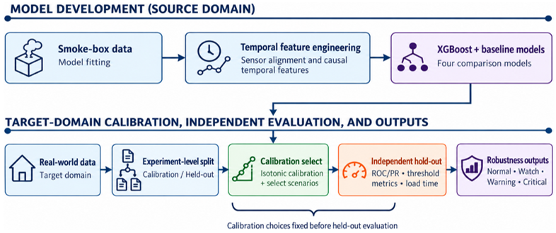
The study makes four principal methodological contributions (Figure 1):
Cross-domain calibration. A two-stage pipeline calibrates smoke-box-trained XGBoost outputs to room-scale target-domain conditions using isotonic regression while preserving an independent experiment-level hold-out set for final evaluation.
Multi-resolution temporal feature engineering. The framework derives 68 predictors from four sensor modalities using instantaneous values, temporal differences, slopes, and rolling summaries at three trailing-window scales.
Experiment-level pre-alarm threshold-crossing timing. The interval between the first calibrated-score threshold crossing and conventional alarm activation is quantified descriptively, enabling consistent temporal comparison across experiments without redefining correctness under the fixed 10-s supervised target.
Calibration-informed risk-state representation. Calibration-only screening is used to map continuous scores to Normal, Watch, Warning, and Critical visualization states, improving interpretability without presenting the mapping as a validated safety-control policy.
Figure 1. Analytical workflow of the proposed pre-alarm fire-risk framework
Figure 1 summarizes the analytical progression from multi-sensor experimental data and temporal feature engineering to model development, target-domain calibration, independent hold-out evaluation, and interpretable risk-state outputs.
3.1 Data sources, experimental datasets, and preprocessing
We used data from the publicly available NIST Smoke Alarm Performance dataset, which provides smoke-box and room-scale experimental smoke-alarm performance data relevant to fire development and alarm activation [1]. The smoke-box experiments were used for model development, whereas the room-scale experiments formed the target domain for probability calibration and independent hold-out evaluation under larger-scale experimental conditions.
The supervised target was defined as a fixed-horizon future-alarm indicator. For each time-indexed observation, alarm_after_10s represents the conventional alarm state 10 time steps ahead, y(t) = alarm(t + 10), computed independently within each experiment using a group-wise forward shift of the raw alarm column. Under the nominal one-second sampling interval, this corresponds to an approximately 10-s forecasting horizon. Smoke-box observations for which a future target value was unavailable were excluded, accounting for the reduction from 184,365 raw observations to 179,795 modeling observations. This formulation embeds the forecasting horizon directly within the supervised-learning task.
After construction of the future-alarm target and alignment of the common variables, the smoke-box modeling dataset contained 179,795 time-indexed observations from 457 experiments, including 14,919 positive target observations (8.3%). The room-scale dataset contained 18,700 observations from 18 experiments, including 11,778 positive target observations (63.0%). Seven room-scale experiments (7,034 observations) were reserved for probability calibration, and 11 experiments (11,666 observations) formed the independent hold-out set. Table 1 summarizes the analysis datasets.
Each experiment file was brought into a consistent tabular form, with time in seconds and an experiment ID to uniquely identify observations. To ensure consistency between the training and external validation domains, only variables common to both were considered. A total of four features were selected: (i) transmittance percentage, (ii) smoke obscuration per foot, (iii) microphone (MIC) signal response, and (iv) carbon monoxide (CO) concentration. The binary microphone indicator was removed due to inconsistent information across domains, which would have affected cross-domain validation.
Table 1. Summary of experimental datasets used for model development, calibration, and evaluation
|
Dataset |
Observations |
Experiments |
Positive Target Rows |
Positive Proportion |
|
Smoke-box modeling data |
179795 |
457 |
14919 |
0.083 |
|
Room-scale experiments |
18700 |
18 |
11778 |
0.630 |
3.2 Temporal feature engineering
Fire development is dynamic; therefore, instantaneous measurements were augmented with causal temporal descriptors computed separately within each experiment. The final 68-predictor specification comprised four raw sensor variables; first differences at lags 1 and 3; short-term slopes over 5 and 10 observations; and rolling mean, minimum, maximum, and standard deviation over trailing windows of 5, 10, and 20 observations. These transformations represent recent signal level, direction, and variability without requiring a recurrent architecture.
The trailing windows of 5, 10, and 20 observations balance responsiveness with stability. Short windows preserve rapid changes, whereas longer windows capture accumulation and attenuate brief fluctuations. The window lengths define local feature context and do not define the separate descriptive threshold-crossing-to-alarm interval.
First-order difference feature:
$\Delta x_i(t)=x_i(t)-x_i(t-1)$ (1)
where, xᵢ(t) = value of sensor variable i at time t; Δxᵢ(t) = first-order temporal difference (rate of change) of sensor i at time t.
Short-term slope feature:
$S_i^w(t)=\frac{x_i(t)-x_i(t-w)}{w}$ (2)
where, w ∈ {5, 10} observations for the short-term slope features; Sᵢⁿ(t) = mean rate of change of sensor i over the preceding w time steps.
Rolling mean feature:
$\mu_i{ }^w(t)=\frac{1}{w} \sum_{k=0}^{w-1} x_i(t-k)$ (3)
where, μᵢⁿ(t) = rolling arithmetic mean of sensor i over window w; k = lag index ranging from 0 (current time) to w−1 (oldest in window).
Rolling minimum, maximum, and standard deviation:
$\begin{aligned} & \min _i{ }^w(t)=\min \left\{x_i(t-k): k=0, \ldots, w-1\right\} \\ & \max _i{ }^w(t)=\max \left\{x_i(t-k): k=0, \ldots, w-1\right\}\end{aligned}$ (4)
where, σᵢⁿ(t) = rolling standard deviation, capturing local signal variability.
3.3 Model development, probability calibration, and evaluation design
The XGBoost classifier was chosen as the main classifier, as it can model nonlinear interactions between temporal predictors in structured multi-sensor data. The final model was trained with 700 boosting estimators, a maximum tree depth of 4, a learning rate of 0.03, a row subsampling rate of 0.85, and a column subsampling rate of 0.85, with a minimum weight of each child set to 5, and a regularization term of 2.0 (L2) and 0.1 (L1). The target distribution in the smoke-box was used to calculate scale_pos_weight to prevent class imbalance. Logistic regression, random forest, linear Support Vector Machine (SVM), and a calibration-derived multi-sensor threshold rule were applied as baseline comparisons with the evaluation design of the experiment.
Features were standardized using a z-score scaler fitted exclusively on the smoke-box training data. The fitted scaler was then applied without refitting to the room-scale calibration and hold-out subsets. The XGBoost trees were not fitted using room-scale observations; they were only fitted using the calibration subset for calibration of the probabilities. Baseline models, preprocessing, and calibration were developed by following scikit-learn compatible workflows [21].
Full configuration details for each comparator are as follows. The logistic regression was computed with the liblinear solver, balanced class weighting, a maximum of 4,000 iterations and default L2 regularization (C = 1.0). Random forest had a total of 500 trees, maximum depth was unlimited, minimum split was 10, minimum leaf was 5 and balanced class weighting was applied. Linear SVM was implemented with C = 1.0, balanced class weighting and max iterations = 30,000. The four per-sensor binary conditions (obscuration ≥ 0.070 %/ft, CO ≥ 0.000, MIC acoustic pressure ≥ 78.42 Pa, transmittance ≤ 99.66%) were combined to an average score, each sensor threshold was determined for every sensor by its 25th percentile (75th percentile for transmittance) of the sensor value in the positive-target calibration-subset observations and the threshold of the rule itself (0.55) was optimized by maximizing the F1-score over 21 evenly spaced candidate thresholds on the calibration subset. Each of the four learned models (logistic regression, random forest, linear SVM, XGBoost) was calibrated on the same seven experiments of the room-scale calibration set, with prefit calibration being applied to all of them. Logistic regression, random forest and XGBoost were prefit calibrated using isotonic regression, while linear SVM was prefit calibrated using sigmoid (Platt) calibration, owing to its non-probabilistic margin-based output and limited number of calibration experiments. Logistic regression, random forest, linear SVM and XGBoost were assessed at a common 0.50 classification threshold, while the sensor-rule baseline was evaluated at its independently determined 0.55 classification threshold.
Smoke-box and room-scale experiments differed in scale, target prevalence (8.3% versus 63.0%), and sensor-response characteristics. Isotonic regression was therefore fitted on the seven-experiment room-scale calibration subset to transform raw XGBoost outputs into calibrated risk scores. Calibration did not alter the fitted XGBoost trees. Because calibration estimates based on finite validation data may be sensitive to sampling variability, the resulting calibration should be interpreted cautiously [22].
The remaining 11 room-scale experiments formed the independent hold-out subset. All final performance metrics were calculated only on these hold-out experiments. The operating classification threshold, θ = 0.50, was specified before hold-out evaluation and was not retrospectively selected from hold-out results.
3.4 Evaluation metrics and exploratory threshold crossing timing analysis
Discrimination was quantified using the area under the Receiver Operating Characteristic–Area Under the Curve (ROC-AUC) and the area under the Precision-Recall–Area Under the Curve (PR-AUC). ROC analysis is widely used to assess classifier discrimination [23], whereas precision-recall analysis is particularly informative for imbalanced classification problems in which the positive class is of primary interest [24]. Threshold-dependent performance was assessed using accuracy, precision, recall, specificity, F1-score, and confusion-matrix counts.
Precision:
$Precision=\frac{T P}{T P+F P}$ (5)
where, TP = true positives (correctly predicted alarm states); P = false positives (non-alarm states incorrectly predicted as alarm).
Recall (Sensitivity):
$Recall=\frac{T P}{T P+F N}$ (6)
where, FN = false negatives (alarm states incorrectly predicted as non-alarm).
F1-score:
$F 1=\frac{2 \times \text { Precision } \text { × } \text { Recall }}{\text { Precision }+ \text { Recall }}$ (7)
Pre-alarm threshold crossing to alarm interval:
$\Delta T_{\text {lead}}=T_{\text {alarm}}-T_{\text {alert}}$ (8)
where, Talarm = time of conventional alarm activation (seconds from experiment onset); Talert = first time at which the calibrated risk score crosses the operating threshold; here, the term alert is shorthand for a score-threshold crossing and does not itself denote a correct fixed-horizon prediction.
A positive ΔTlead indicates that the first threshold crossing occurred before conventional alarm activation, whereas zero or a negative value indicates a first crossing at or after alarm activation. The interval in Eq. (8) is used only as an exploratory descriptive timing quantity and does not alter classification correctness under the fixed-horizon supervised task. Under y(t) = alarm(t + 10), a pre-alarm threshold crossing occurring more than 10 s before conventional alarm activation corresponds to a negative target and is therefore a false-positive classification in the primary supervised evaluation. Accordingly, Eq. (8) is not interpreted as a verified fixed-horizon predictive lead.
3.5 Data-driven risk-state representation
A data-driven risk-state layer was constructed by augmenting each time-indexed room-scale observation with the calibrated model score R(t), a discrete visualization state, and a corresponding decision-support recommendation. This layer will not create synthetic fire scenarios, simulate ignition physics, keep a live connection with a physical building, or be controlled in any way. It is used to show an approximation of risk over time in the experimental data.
The visualization-state boundaries were not adopted as universal probability cut-offs. Only the room-scale calibration subset was used to compare candidate configurations prior to independent hold-out evaluation. Screening included: Representing all four states, avoiding a single-state dominance, ordered progression, maintaining pre-alarm occurrence of the Warning and Critical states, and minimizing unnecessary short-duration switching. The chosen boundaries (0.350, 0.500 and 0.725) were established prior to their application to the independent hold-out set. No hold-out observations or hold-out performance metrics were used for the boundary selection. These are data-derived visualization-state boundaries, and not fire-safety thresholds or regulatory action levels.
The screening procedure searched a candidate grid of 15 lower-boundary values from 0.100 to 0.450 (step 0.025) and 17 upper-boundary values from 0.550 to 0.950 (step 0.025), with the middle boundary fixed at 0.500, yielding 15 × 17 = 255 candidate configurations satisfying lower < 0.500 < upper. Each configuration was evaluated exclusively on the seven-experiment calibration subset and retained as feasible only if it satisfied four constraints: every state occupied at least 5% of calibration observations; no state occupied more than 70%; the Critical state was reached before alarm activation in at least 70% of alarm-producing calibration experiments; and the Warning state preceded or coincided with the Critical state in every experiment. Of the 255 candidates, 135 satisfied all four constraints. Feasible configurations were ranked lexicographically by (1) minimum transitions per 1,000 observations, (2) maximum of the minimum state-occupancy fraction, (3) maximum median state-run duration, and (4) maximum median Critical-state threshold crossing to alarm interval; the top-ranked configuration (0.350, 0.500, 0.725) was retained as the final boundary specification.
Relative to the equally spaced reference configuration, the selected configuration reduced total transitions by 64 (15.8%) and transitions per 1,000 observations from 57.58 to 48.48. It also increased the median state-run duration from 3.0 to 5.0 s and improved the minimum state occupancy from 14.19% to 16.02%, while preserving the critical pre-alarm threshold crossing rate at 0.714 and maintaining pre-alarm Warning-state occurrence. The selected configuration was therefore retained because it improved temporal stability and state representation without sacrificing calibration-subset pre-alarm behavior. The boundary comparison and state mapping are summarized in Tables 2 and 3, respectively.
The resulting state log is a derived time-resolved dataset containing the experiment identifier, timestamp, calibrated risk score, visualization state, and recommended response. It supports analysis of transitions, state occupancy, and the timing of elevated risk relative to conventional alarm activation. The framework is therefore described as digital-twin-oriented rather than as a complete physics-based or cyber-physical digital twin.
Table 2. Calibration-only comparison of the equally spaced reference configuration and the calibration-set-selected risk-state boundaries
|
Metric |
Equally Spaced Reference |
Calibration-Set Selected |
|
Boundaries |
0.250 / 0.500 / 0.750 |
0.350 / 0.500 / 0.725 |
|
Total transitions |
405 |
341 |
|
Transitions per 1,000 observations |
57.58 |
48.48 |
|
Median state-run duration (s) |
3.0 |
5.0 |
|
Minimum state occupancy (%) |
14.19 |
16.02 |
|
Critical pre-alarm threshold crossing rate |
0.714 |
0.714 |
Table 3. Calibration-set-selected risk-state visualization mapping based on calibrated score R(t)
|
Risk Level |
Score R(t) |
Risk-State Interpretation |
Decision-Support Action |
|
Normal |
R(t) < 0.350 |
No elevated visualization-state pattern detected |
Continue monitoring |
|
Watch |
0.350 ≤ R(t) < 0.500 |
Lower-level evolving risk pattern |
Increase monitoring attention |
|
Warning |
0.500 ≤ R(t) < 0.725 |
Elevated pre-alarm risk pattern |
Notify safety operator |
|
Critical |
R(t) ≥ 0.725 |
Strong elevated risk pattern |
Consider pre-alarm intervention |
4.1 Model discrimination and calibration performance
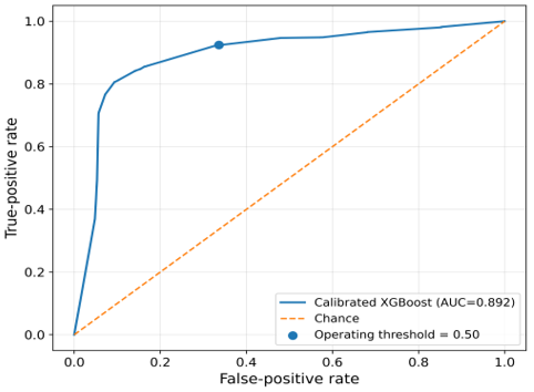
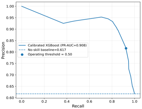
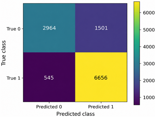
Following isotonic calibration on the room-scale calibration subset, XGBoost achieved ROC-AUC = 0.892 and PR-AUC = 0.908 on the independent hold-out set (Table 4). At θ = 0.50, accuracy was 0.825, precision was 0.816, recall was 0.924, specificity was 0.664, and F1-score was 0.867. The confusion matrix contained 2,964 true negatives, 1,501 false positives, 545 false negatives, and 6,656 true positives. These values quantify performance within the controlled room-scale experiments and do not establish operational building performance.
Table 4. Performance of calibrated Extreme Gradient Boosting (XGBoost) on the independent room-scale hold-out set
|
Threshold |
ROC-AUC |
PR-AUC |
Accuracy |
Precision |
Recall |
F1 |
|
0.500 |
0.892 |
0.908 |
0.825 |
0.816 |
0.924 |
0.867 |
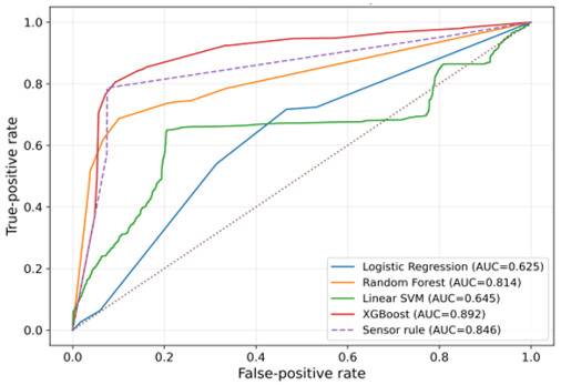
XGBoost achieved the highest ROC-AUC, PR-AUC, and F1-score. The simple sensor-rule baseline achieved the highest accuracy, precision, and specificity and the fewest false-positive rows, whereas linear SVM achieved the highest recall and the fewest false-negative rows but exhibited extremely low specificity.
Comparative evaluation (Table 5 and Figure 2) showed that XGBoost achieved the highest ROC-AUC, PR-AUC, and F1-score. Figures 3–5 show the calibrated XGBoost ROC curve, precision-recall curve, and confusion matrix. The sensor-rule baseline achieved the highest accuracy, precision, and specificity, with only 336 false-positive rows, but produced 1,537 false negatives. Linear SVM achieved the highest recall and only 339 false negatives, but its specificity was 0.051, with 4,236 false positives. These results quantify the trade-off between early-risk sensitivity and conservative alerting.
Table 5. Comparative performance of calibrated Extreme Gradient Boosting (XGBoost) and baseline models on the independent room-scale hold-out set
|
Model |
ROC-AUC |
PR-AUC |
Precision |
Recall |
Specificity |
F1 |
Accuracy |
FP |
FN |
|
Logistic Regression |
0.625 |
0.694 |
0.712 |
0.717 |
0.532 |
0.715 |
0.646 |
2089 |
2037 |
|
Random Forest |
0.814 |
0.866 |
0.823 |
0.745 |
0.742 |
0.782 |
0.744 |
1153 |
1836 |
|
SVM |
0.645 |
0.775 |
0.618 |
0.953 |
0.051 |
0.750 |
0.608 |
4236 |
339 |
|
XGBoost |
0.892 |
0.908 |
0.816 |
0.924 |
0.664 |
0.867 |
0.825 |
1501 |
545 |
|
Simple sensor-rule baseline |
0.846 |
0.869 |
0.944 |
0.787 |
0.925 |
0.858 |
0.839 |
336 |
1537 |
Figure 2. ROC comparison of calibrated Extreme Gradient Boosting (XGBoost) and baseline models on the independent room-scale hold-out set
Figure 3. ROC curve of calibrated Extreme Gradient Boosting (XGBoost) on the independent room-scale hold-out set (ROC-AUC = 0.892)
Figure 4. Precision-recall curve of calibrated Extreme Gradient Boosting (XGBoost) on the independent room-scale hold-out set (PR-AUC = 0.908)
Figure 5. Confusion matrix of calibrated Extreme Gradient Boosting (XGBoost) at θ = 0.50
4.2 Operating-threshold sensitivity and visualization-state boundary selection
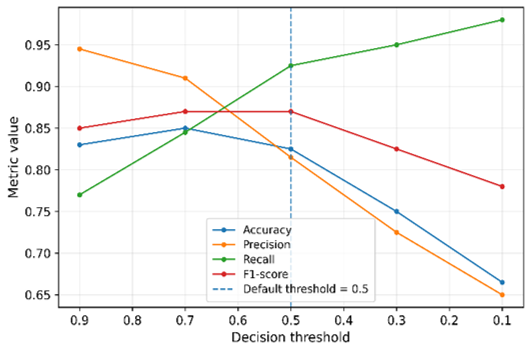
Sensitivity analysis across operating classification thresholds from 0.10 to 0.90 characterized the precision-recall trade-off while retaining $\theta$ = 0.50 as the primary operating point. At $\theta$ = 0.70, accuracy and F1-score increased to 0.848 and 0.872, respectively, with precision 0.907 and recall 0.840. Precision rose to 0.945 and specificity to 0.928 at $\theta$ = 0.90, with a decrease in recall to 0.766. At $\theta$ = 0.10, the recall was 0.980, and the specificity was 0.151. The alternative operating thresholds are not for the primary hold-out result but only for sensitivity characterization.
Operating-threshold sensitivity (Table 6 and Figure 6) was evaluated separately from calibration-only visualization-state boundary selection. The selected state mapping reduced calibration-set transitions by 15.8%, from 405 to 341, corresponding to a decrease from 57.58 to 48.48 transitions per 1,000 observations. Median state-run duration increased from 3.0 to 5.0 s, minimum state occupancy increased from 14.19% to 16.02%, and the Critical pre-alarm threshold crossing rate remained 0.714, while pre-alarm Warning state occurrence was preserved. These results support the selected boundaries as a more stable and better-balanced calibration-set configuration; they do not represent regulatory or operational thresholds.
Table 6. Operating-threshold sensitivity of calibrated Extreme Gradient Boosting (XGBoost) on the room-scale hold-out set; $\theta$ = 0.50 is the primary operating point
|
$\theta$ |
Accuracy |
Precision |
Recall |
F1 |
TN |
FP |
FN |
TP |
|
0.900 |
0.828 |
0.945 |
0.766 |
0.846 |
4145 |
320 |
1684 |
5517 |
|
0.700 |
0.848 |
0.907 |
0.840 |
0.872 |
3843 |
622 |
1151 |
6050 |
|
0.500 |
0.825 |
0.816 |
0.924 |
0.867 |
2964 |
1501 |
545 |
6656 |
|
0.300 |
0.747 |
0.726 |
0.949 |
0.823 |
1888 |
2577 |
370 |
6831 |
|
0.100 |
0.663 |
0.651 |
0.980 |
0.782 |
674 |
3791 |
141 |
7060 |
Figure 6. Threshold sensitivity of calibrated Extreme Gradient Boosting (XGBoost)
4.3 Feature importance analysis
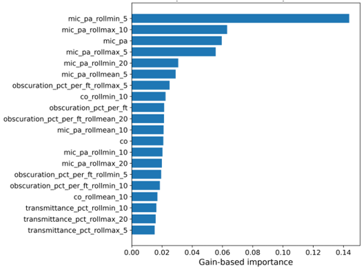
Table 7 and Figure 7 show the gain-based feature importance in XGBoost, where most of the features were related to microphone acoustic pressure. The most significant predictor was mic_pa_rollmin_5 (0.144), followed by mic_pa_rollmax_10 (0.063), instantaneous mic_pa (0.060), and mic_pa_rollmax_5 (0.056). Leading features were also optical obscuration and CO predictors, further indicating complementary roles for acoustic, optical, and chemical measurements.
Table 7. Top 10 Extreme Gradient Boosting (XGBoost) feature importances (gain-based) for the calibrated model pipeline
|
Feature |
Importance Score (Gain) |
|
mic_pa_rollmin_5 |
0.144 |
|
mic_pa_rollmax_10 |
0.063 |
|
mic_pa |
0.060 |
|
mic_pa_rollmax_5 |
0.056 |
|
mic_pa_rollmin_20 |
0.031 |
|
mic_pa_rollmean_5 |
0.029 |
|
obscuration_pct_per_ft_rollmax_5 |
0.025 |
|
co_rollmin_10 |
0.022 |
|
obscuration_pct_per_ft |
0.021 |
|
obscuration_pct_per_ft_rollmean_20 |
0.021 |
Figure 7. Top 20 gain-based Extreme Gradient Boosting (XGBoost) feature importances
The contribution of rolling mean features of smoke obscuration, optical transmittance, and CO concentration was also significant, and together they expressed the rationale of our multi-sensor system design. The use of acoustic sensors and optical/chemical sensors, as well as the time diversity of their properties, is consistent with the assumption that the temporal evolution of the acoustic, optical, and chemical properties will differ depending on the combustion conditions.
4.4 Exploratory pre-alarm threshold crossing timing analysis
The temporal behavior of the calibrated score was explored using the interval defined in Eq. (8) for each room-scale hold-out experiment in which the conventional alarm activated. In this analysis, the quantity is used solely as a descriptive interval from the first threshold crossing to subsequent conventional alarm activation; it is not a fixed-horizon forecasting metric and does not reclassify out-of-horizon crossings as correct predictions.
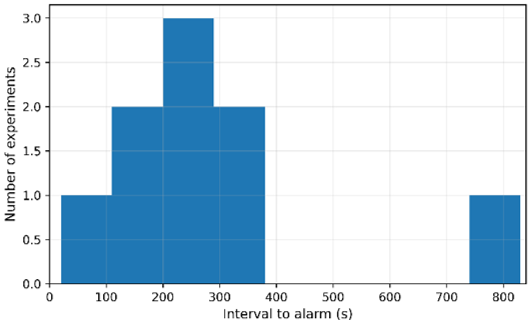
Of the 11 alarm-producing room-scale hold-out experiments, 9 (81.8%) exhibited a threshold crossing before conventional alarm activation, whereas in 2 experiments the first crossing occurred at or after alarm activation. Among the 9 experiments with a pre-alarm threshold crossing, the median descriptive threshold crossing to alarm interval was 214.0 s (IQR 193.0-304.0 s), the mean was 277.1 s, and the observed range was 17–819 s. The exact 95% confidence interval for the 9/11 experiment-level pre-alarm threshold crossing proportion was 48.2%–97.7%, reflecting the limited number of independent experiments (Tables 8–10 and Figure 8).
Table 8. Aggregate pre-alarm threshold crossing timing summary for the room-scale hold-out experiments
|
Total Alarm Experiments |
Pre-alarm Threshold Crossing |
First Crossing At/After Alarm |
Pre-alarm Crossing Proportion |
|
11 |
9 |
2 |
0.818 (81.8%) |
Table 9. Threshold crossing-to-alarm interval summary statistics for experiments with a pre-alarm crossing (n = 9)
|
Pre-alarm Crossing (n) |
Median Interval to Alarm (s) |
Q1 (s) |
Q3 (s) |
Mean Interval to Alarm (s) |
|
9 |
214.0 |
193.0 |
304.0 |
277.1 |
Table 10. Experiment-level timing of first pre-alarm threshold crossings in room-scale hold-out experiments
|
Experiment |
Alarm Time (s) |
First Crossing (s) |
Interval to Alarm (s) |
|
FryHBG1T1 |
256 |
11 |
245 |
|
FryHBG2T1 |
221 |
11 |
210 |
|
FryHBG3T1 |
225 |
11 |
214 |
|
FryHBG4T1 |
224 |
31 |
193 |
|
SFG2T1 |
371 |
67 |
304 |
|
SFG5T1 |
341 |
11 |
330 |
|
SFoamG5T1 |
831 |
12 |
819 |
|
ToastG2T1 |
183 |
166 |
17 |
|
ToastG3T1 |
201 |
39 |
162 |
Figure 8. Distribution of pre-alarm threshold crossing to alarm intervals
The two experiments without a pre-alarm threshold crossing were SFoamG1T1 and SFoamG3T1, with first threshold crossings 84 s and 117 s after conventional alarm activation, respectively. Their delayed threshold crossings and the wide experiment-level variability motivate evaluation across additional fuels, non-alarm trials, and larger independent datasets.
4.5 Representative dynamic risk timelines
Dynamic risk-score timelines illustrate the temporal progression of calibrated risk estimates prior to conventional alarm activation. Two contrasting representative experiments are examined.
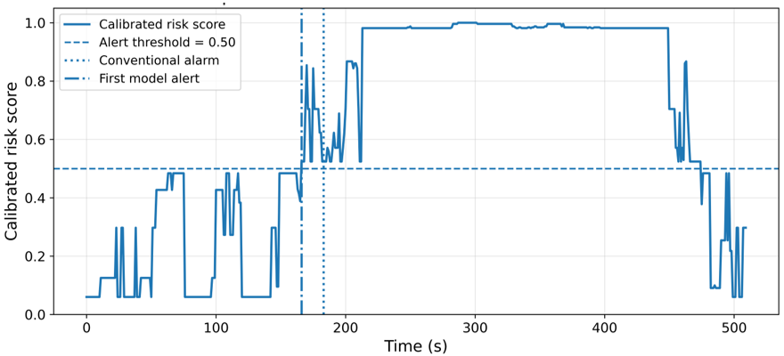
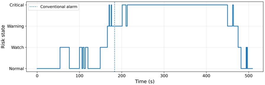
ToastG2T1 provides the smallest positive pre-alarm threshold crossing interval in the descriptive timing analysis: the calibrated score crossed θ = 0.50 at 166 s, 17 s before conventional alarm activation at 183 s (Figure 9). This experiment illustrates near-alarm risk-score escalation with limited temporal separation from alarm activation.
Figure 9. Dynamic risk-score timeline for ToastG2T1 (first threshold crossing 17 s before conventional alarm)
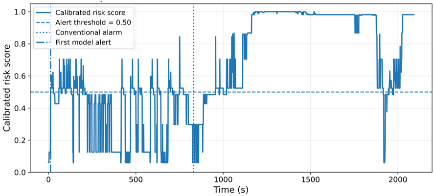
SFoamG5T1 exemplifies an extended pre-alarm threshold-crossing interval: the first model threshold crossing occurred at 12 s and conventional alarm activation at 831 s, giving a descriptive interval of 819 s (Figure 10). Under the fixed 10-s target, the crossing at t = 12 s corresponds to y(12) = alarm(22) = 0 and is therefore a false-positive classification in the primary supervised task. The 819-s value is retained only as an exploratory description of the time between the first threshold crossing and the later conventional alarm; it is not a correct 10-s-ahead forecast.
Figure 10. Dynamic risk-score timeline for SFoamG5T1 (first threshold crossing 819 s before conventional alarm)
Several experiments produced threshold crossings near the beginning of the observation period. FryHBG1T1, FryHBG2T1, FryHBG3T1, SFG5T1, and SFoamG5T1 first crossed θ = 0.50 at 11-12 s. These cases were retained in the exploratory timing analysis but should be interpreted cautiously because the available pre-crossing baseline was brief.
4.6 Risk-State layer results
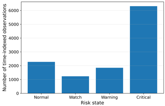
The 11,666 hold-out observations were converted into a time-resolved risk-state log using the calibration-set-selected boundaries in Table 3. Overall, 2,277 observations were classified as Normal, 1,232 as Watch, 1,847 as Warning, and 6,310 as Critical. Experiment-level state-transition counts ranged from 14 to 152 under the final mapping.
The risk-state layer exhibited a pre-alarm threshold crossing in 9 of 11 alarm-producing experiments, while in 2 experiments the first threshold crossing occurred at or after conventional alarm activation. Median and mean pre-alarm threshold crossing-to-alarm intervals were 214.0 s and 277.1 s, respectively. These quantities are descriptive timing statistics and are distinct from the fixed 10-s supervised forecasting evaluation. All experiments reached the Critical visualization state, consistent with the alarm-producing composition of the hold-out set (Tables 11, 12, and Figures 11–13).
Because the independent hold-out subset contained no complete non-alarm experiments, experiment-level false pre-alarm performance was not estimable. Row-level false positives (n = 1,501) quantify time-indexed classification errors and should not be interpreted as complete experiment-level false alarms.
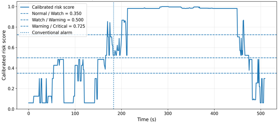
Figures 12 and 13 show the ToastG2T1 continuous risk-score and state-transition timelines using the selected boundaries of 0.350, 0.500, and 0.725. The visualization provides an auditable summary of changing calibrated risk but is not a validated operational control policy.
The risk-state output supplements the continuous probability score with a graded monitoring label and illustrative decision-support recommendation. Its operational usefulness requires prospective evaluation with non-alarm scenarios, real-time implementation, human-factors assessment, and external building data.
Table 11. Risk-state and threshold crossing timing summary across 11 room-scale hold-out experiments
|
Metric |
Value |
|
Number of room hold-out experiments |
11 |
|
Total time-indexed observations |
11666 |
|
Experiments with pre-alarm threshold crossing |
9 |
|
First threshold crossing at or after alarm activation |
2 |
|
Experiment-level false pre-alarm rate |
Not estimable (no non-alarm hold-out experiments) |
|
Median pre-alarm interval to alarm (s) |
214.0 |
|
Mean pre-alarm interval to alarm (s) |
277.1 |
|
Risk-state boundaries |
0.350 / 0.500 / 0.725 |
Table 12. Experiment-level threshold crossing timing and state-transition summary for the room-scale hold-out set
|
Experiment |
Alarm (s) |
First Crossing (s) |
Interval to Alarm (s) |
Max State |
State Transitions |
Crossing Timing |
|
FryHBG1T1 |
256 |
11 |
245 |
Critical |
29 |
Pre-alarm |
|
FryHBG2T1 |
221 |
11 |
210 |
Critical |
24 |
Pre-alarm |
|
FryHBG3T1 |
225 |
11 |
214 |
Critical |
48 |
Pre-alarm |
|
FryHBG4T1 |
224 |
31 |
193 |
Critical |
27 |
Pre-alarm |
|
SFG2T1 |
371 |
67 |
304 |
Critical |
15 |
Pre-alarm |
|
SFG5T1 |
341 |
11 |
330 |
Critical |
24 |
Pre-alarm |
|
SFoamG1T1 |
924 |
1,008 |
-84 |
Critical |
152 |
At/after alarm |
|
SFoamG3T1 |
805 |
922 |
-117 |
Critical |
76 |
At/after alarm |
|
SFoamG5T1 |
831 |
12 |
819 |
Critical |
104 |
Pre-alarm |
|
ToastG2T1 |
183 |
166 |
17 |
Critical |
26 |
Pre-alarm |
|
ToastG3T1 |
201 |
39 |
162 |
Critical |
14 |
Pre-alarm |
Figure 11. Distribution of selected risk-state labels in the hold-out set
Figure 12. Calibrated risk-score timeline for ToastG2T1 using boundaries 0.350, 0.500, and 0.725
Figure 13. Selected visualization-state transitions for ToastG2T1
The calibrated XGBoost model achieved ROC-AUC = 0.892 and PR-AUC = 0.908 on the independent room-scale hold-out set, indicating substantial discrimination despite the domain difference between smoke-box training and room-scale evaluation. A split and separate target-domain calibration subset is employed to minimize direct information flow between model development and final evaluation, but the number of room-scale experiments is limited, thus limiting the ability to generalize.
The model outputs were calibrated to the room-scale calibration subset by using isotonic calibration. The findings indicate that target domain calibration could be appropriate for cases where representative target data can be found; however, the present study does not generalize the results to operational buildings, and the small calibration sample size restricts general conclusions about transferability.
A calibration-only boundary comparison is used to select the final configuration with a basis of a reference configuration equally spaced. The chosen configuration reduced transition frequency and extended median state runs, and maintained calibration-subset pre-alarm state occurrence. These enhancements are related to temporal stability and state occupancy but are limited to seven calibration experiments and are not definitive state thresholds for other sensors, fuels, or buildings.
At θ = 0.50, the recall, precision, and specificity of XGBoost were 0.924, 0.816, and 0.664, respectively, and the number of false-negative and false-positive rows were 545 and 1,501, respectively. The sensor rule yielded a smaller number of false-positive rows, but a significantly higher number of false-negative rows (1,537) compared with linear SVM (4,236 false-positive rows, specificity 0.051). The comparison is thus not a general superiority of one approach over the others but rather displays different error profiles.
The baseline comparison does not assert that one or the other is better in every situation, but rather helps to be nuanced in interpreting the findings. XGBoost showed the best discrimination and F1-score; linear SVM had the highest recall but more rows of false-positive burden; and the sensor-rule baseline had the best precision, specificity, and overall accuracy, but with more rows of false positives. The trade-off will be specific to each operation, depending on how much the missed risk and nuisance messages will cost the operation, and needs to be determined in advance.
The issue of discrimination was also discussed, because rolling obscuration and CO features also had a role to play. The feature importance analysis is not causal and does not indicate resilience to sensor failure.
This dataset includes the presence of local temporal context, with the relative importance of temporal statistics over instantaneous values. Nevertheless, mechanistic interpretations should be taken with a pinch of salt, as it is not a causal combustion process that can be determined by gain-based feature importance.
The results of the 11 experiments show that, in these controlled room-scale experiments, calibrated-score threshold crossings occurred before conventional alarm activation in 9 experiments, with a median descriptive threshold crossing to alarm interval of 214.0 s. This timing statistic is separate from, and should not be interpreted as, the fixed 10-s supervised forecasting horizon. The width of the confidence interval was broad, and the result is not intended to be extrapolated to gains in evacuation time or operational benefit for occupied buildings.
There was a high degree of fuel-experimental condition heterogeneity, with descriptive threshold-crossing-to-alarm intervals ranging from 17 to 819 s. Long intervals can indicate early elevation of the calibrated score relative to later conventional alarm activation, but they do not establish correct fixed-horizon forecasts or practical usefulness and do not demonstrate avoidance of "alarm fatigue" without non-alarm trials and an independently verified response policy.
The two late-detected synthetic-foam experiments and the huge range in experiments highlight the need for more fuel types, non-fire experiments, more independent experiments, and external validation. It is therefore recommended that further investigation be done before making conclusions at the deployment level for the present findings.
This study presents a proof-of-concept framework combining 68 multi-sensor temporal predictors, calibrated XGBoost risk scoring, comparative baseline evaluation, and an interpretable risk-state representation. On the independent room-scale hold-out set, XGBoost achieved ROC-AUC = 0.892, PR-AUC = 0.908, and F1-score = 0.867. Among the nine alarm-producing experiments with a pre-alarm threshold crossing, the median descriptive threshold crossing-to-alarm interval was 214.0 s; this exploratory quantity is distinct from the fixed 10-s supervised forecasting horizon.
Data-informed visualization boundaries of 0.350, 0.500, and 0.725 were selected using calibration-only screening against an equally spaced reference configuration.
Larger and more varied fire and non-fire datasets, full-scale and multi-zone building experiments, calibration and state-boundary validation in separate external cohorts, computational testing under real-time conditions, human-factors assessment, and incorporation of physical sensing and building-management systems should be incorporated into future research. As a research prototype and a part of a future digital-twin safety system, the framework should not be regarded as a deployable smart-building safety system until such information is available.
[1] National Institute of Standards and Technology (NIST). (2016). Data on smoke alarm performance: A compilation to NIST TN 1947. https://www.nist.gov/el/fire/engineered-fire-safety/data-smoke-alarm-performance.
[2] Cleary, T.G. (2016). A study on the performance of current smoke alarms to the new fire and nuisance tests prescribed in ANSI/UL217-2015 (NIST Technical Note 1947). US Department of Commerce, National Institute of Standards and Technology. https://doi.org/10.6028/NIST.TN.1947
[3] Ronchi, E., Nilsson, D. (2013). Fire evacuation in high-rise buildings: A review of human behaviour and modelling research. Fire Science Reviews, 2(1): 7. https://doi.org/10.1186/2193-0414-2-7
[4] Lovreglio, R., Fonzone, A., Dell’Olio, L. (2016). A mixed logit model for predicting exit choice during building evacuations. Transportation Research Part A: Policy and Practice, 92: 59-75. https://doi.org/10.1016/j.tra.2016.06.018
[5] Li, X., Vázquez-López, A., Sánchez del Río Sáez, J., Wang, D.Y. (2022). Recent advances on early-stage fire-warning systems: Mechanism, performance, and perspective. Nano-Micro Letters, 14(1): 197. https://doi.org/10.1007/s40820-022-00938-x
[6] Shaharuddin, S., Maulud, K.N.A., Rahman, S.A.F.S.A., Ani, A.I.C., Pradhan, B. (2023). The role of IoT sensors in smart building context for indoor fire hazard scenario: A systematic review of interdisciplinary articles. Internet of Things, 22: 100803. https://doi.org/10.1016/j.iot.2023.100803
[7] Wu, L., Chen, L., Hao, X. (2021). Multi-sensor data fusion algorithm for indoor fire early warning based on BP neural network. Information, 12(2): 59. https://doi.org/10.3390/info12020059
[8] Grieves, M., Vickers, J. (2017). Digital twin: Mitigating unpredictable, undesirable emergent behavior in complex systems. In Transdisciplinary Perspectives on Complex Systems: New Findings and Approaches, Cham: Springer, pp. 85-113. https://doi.org/10.1007/978-3-319-38756-7_4
[9] Tao, F., Zhang, H., Liu, A., Nee, A.Y. (2019). Digital twin in industry: State-of-the-art. IEEE Transactions on Industrial Informatics, 15(4): 2405-2415. https://doi.org/10.1109/TII.2018.2873186
[10] Kritzinger, W., Karner, M., Traar, G., Henjes, J., Sihn, W. (2018). Digital twin in manufacturing: A categorical literature review and classification. IFAC-PapersOnline, 51(11): 1016-1022. https://doi.org/10.1016/j.ifacol.2018.08.474
[11] Rasheed, A., San, O., Kvamsdal, T. (2020). Digital twin: Values, challenges and enablers from a modeling perspective. IEEE Access, 8: 21980-22012. https://doi.org/10.1109/ACCESS.2020.2970143.
[12] Boje, C., Guerriero, A., Kubicki, S., Rezgui, Y. (2020). Towards a semantic construction digital twin: Directions for future research. Automation in Construction, 114: 103179. https://doi.org/10.1016/j.autcon.2020.103179
[13] Bentéjac, C., Csörgő, A., Martínez-Muñoz, G. (2021). A comparative analysis of gradient boosting algorithms. Artificial Intelligence Review, 54(3): 1937-1967. https://doi.org/10.1007/s10462-020-09896-5
[14] Chen, T., Guestrin, C. (2016). XGBoost: A scalable tree boosting system. In Proceedings of the 22nd ACM SIGKDD International Conference on Knowledge Discovery and Data Mining, San Francisco, CA, USA, pp. 785-794. https://doi.org/10.1145/2939672.2939785
[15] Niculescu-Mizil, A., Caruana, R. (2005). Predicting good probabilities with supervised learning. In Proceedings of the 22nd International Conference on Machine Learning, Bonn, Germany, pp. 625-632. https://doi.org/10.1145/1102351.1102430
[16] He, H.J., Zhou, Z.H., Sun, Y.B., Li, Q. (2025). Fire risk assessment and simulation of multi-functional teaching buildings: A combined application of DEMATEL and PyroSim. Journal of Engineering Management and Systems Engineering, 4(1): 1-20. https://doi.org/10.56578/jemse040101
[17] Li, Q., Zhou, Z.H., Sun, Y.B., He, H.J. (2024). Fire risk assessment and scenario simulation for employee dormitory buildings. Journal of Operational and Strategic Analytics, 2(3): 193-214. https://doi.org/10.56578/josa020305
[18] Lu, Q., Parlikad, A.K., Woodall, P., et al. (2020). Developing a digital twin at building and city levels: Case study of West Cambridge campus. Journal of Management in Engineering, 36(3): 05020004. https://doi.org/10.1061/(ASCE)ME.1943-5479.0000763
[19] Sun, Q., Turkan, Y. (2020). A BIM-based simulation framework for fire safety management and investigation of the critical factors affecting human evacuation performance. Advanced Engineering Informatics, 44: 101093. https://doi.org/10.1016/j.aei.2020.101093
[20] Lattimer, B.Y., Hodges, J.L., Lattimer, A.M. (2020). Using machine learning in physics-based simulation of fire. Fire Safety Journal, 114: 102991. https://doi.org/10.1016/j.firesaf.2020.102991
[21] Pedregosa, F., Varoquaux, G., Gramfort, A., et al. (2011). Scikit-learn: Machine learning in Python. Journal of Machine Learning Research, 12: 2825-2830. https://www.jmlr.org/papers/v12/pedregosa11a.html.
[22] Lee, D., Huang, X., Hassani, H., Dobriban, E. (2023). T-Cal: An optimal test for the calibration of predictive models. Journal of Machine Learning Research, 24(335): 1-72. https://www.jmlr.org/papers/v24/22-0320.html.
[23] Fawcett, T. (2006). An introduction to ROC analysis. Pattern Recognition Letters, 27(8): 861-874. https://doi.org/10.1016/j.patrec.2005.10.010
[24] Davis, J., Goadrich, M. (2006). The relationship between Precision-Recall and ROC curves. In Proceedings of the 23rd International Conference on Machine Learning, Pittsburgh, PA, USA, pp. 233-240. https://doi.org/10.1145/1143844.1143874