Carlos A. Gutierrez-Acosta | Luis A. Orihuela-Orozco | Brayan S. Ponce-Galarza | Juan Jesús Soria-Quijaite | Nemias Saboya*
© 2026 The authors. This article is published by IIETA and is licensed under the CC BY 4.0 license (http://creativecommons.org/licenses/by/4.0/).
OPEN ACCESS
This study presents a comparative unsupervised workflow combining principal component analysis (PCA) with four clustering algorithms (K-Means, hierarchical agglomerative clustering (H-Clust)), Clustering Large Applications (CLARA), and Density-Based Spatial Clustering (DBSCAN)) to detect anomalous patterns in the UNSW-NB15 dataset. Thirty-nine standardized variables were reduced to ten principal components, preserving 78% of total variance. Guided by the silhouette coefficient, k = 7 clusters was adopted. For a fair comparison, all algorithms were evaluated on a fixed 10,000 record sample, while K-Means was additionally fitted to the complete dataset (n = 82,332). On the complete dataset, K-Means achieved up to 100% purity for Normal traffic and 94.6% for Generic attacks, alongside heterogeneous clusters. Comparatively, K-Means, H-Clust, and CLARA achieved statistically similar, modest alignment with true labels (Adjusted Rand Index (ARI) 0.10-0.13) across random seeds. Conversely, DBSCAN failed to meaningfully partition the traffic (ARI near zero) despite obtaining the highest internal silhouette score, a divergence termed the “DBSCAN paradox.” These findings demonstrate that centroid-, hierarchy-, and medoid-based partitions achieve comparable, seed-sensitive alignment, proving internal cohesion metrics alone are insufficient for cybersecurity evaluation. This PCA-based pipeline offers a promising label-free pre-alert module for security operations centers, though moderate external validity indicates room for improvement.
cybersecurity, threats, cyber attacks, clustering, K-Means
The primary challenge in contemporary cybersecurity lies in effectively detecting attacks amid a constantly mutating threat landscape [1]. Traditionally, Intrusion Detection Systems (IDS) have operated under supervised approaches that require large volumes of labeled data and continuous updates to remain effective [2]; however, this reliance leaves them vulnerable to emerging threats or variants that have not yet been catalogued.
Unsupervised models offer a promising alternative, capable of automatically identifying anomalous or hidden patterns in large-scale datasets [3]. In this context, clustering is particularly suitable, as it groups network traffic into segments of homogeneous behavior without requiring prior labels [4]. Its combination with dimensionality reduction techniques such as principal component analysis (PCA) also enhances data interpretability and facilitates visualization of the results obtained.
Various studies have demonstrated that the application of unsupervised techniques enables the detection of malicious traffic without relying on predefined characteristics, one representative example is the use of geographic-domain and DNS-pattern analysis to detect latent threats [5]. In distributed environments, unsupervised federated learning has been successfully deployed to preserve data privacy while detecting intrusions [6]. These types of strategies are becoming increasingly critical given the rise in encrypted traffic and the use of evasive technologies by attackers, where clustering techniques have detected malicious flows even in TLS connections without prior decryption [7].
Unsupervised models have even shown strong performance in identifying anomalous behaviors in cyber-physical systems and critical infrastructures, where attacks do not follow traditional patterns [8]. In Internet of Things (IoT) networks, hybrid clustering approaches have produced more adaptive detectors by combining local density metrics [9] with anomaly isolation techniques [10].
This work provides a comparative evaluation of four unsupervised clustering algorithms: K-Means, hierarchical agglomerative clustering (H-Clust), Clustering Large Applications (CLARA), and Density-Based Spatial Clustering (DBSCAN), all preceded by dimensionality reduction through PCA and applied to the UNSW-NB15 dataset.
The central objective is to determine which of these models most effectively characterizes the different types of network traffic, distinguishing between normal flows and cyberattacks. Through the structural analysis of the clusters generated by each method, the study seeks to identify the most robust tool for real cybersecurity environments, with the capacity to detect threats early without depending on labeled data.
The study uses the UNSW-NB15 dataset [11], which records a variety of network events, both normal and malicious, including port scans, intrusion attempts, and unauthorized access [12]. This dataset serves as a widely recognized benchmark in cybersecurity research [13]. Data preparation was carried out in R following an exploratory data analysis (EDA) methodology, which included the removal of incomplete records and the transformation of variables to ensure analytical quality. This step is decisive: previous research has shown that rigorous cleaning reduces bias and improves generalization capacity in unsupervised detection models [14]. Of the 49 available attributes, only the 39 quantitative variables in the dataset were selected, mainly related to traffic volume, session times, connection counters, and TCP/UDP protocol flags, because they are representative variables of network behavior [15].
This type of selection has been verified in studies on intrusive networks by focusing on measurable metrics that demonstrate network usage patterns [16]. Subsequently, a cleaning process was applied by removing all rows that contained null values (NA) to ensure the integrity of the analysis. The data were standardized through mean centering and unit variance scaling (z-score), with the aim of neutralizing differences in magnitude among variables [17] and ensuring correct interpretation by the dimensionality reduction model. These types of techniques are important in distance-based models such as K-Means, where scale directly alters clustering [18].
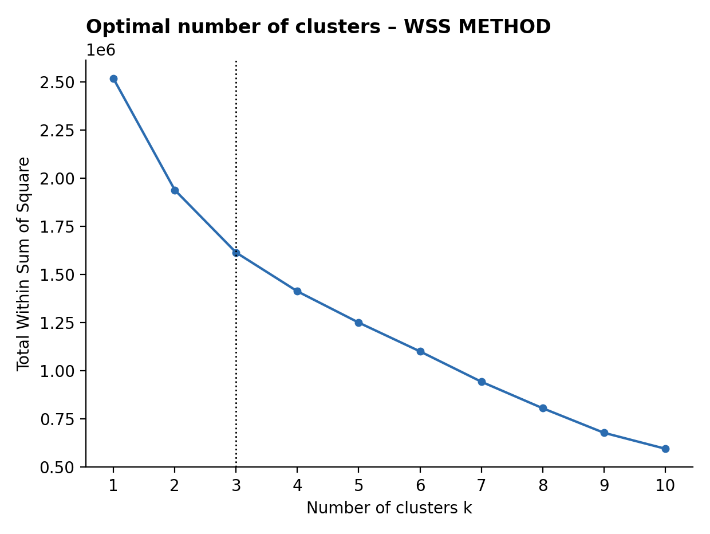
The prcomp function in the R programming environment was employed to perform PCA [19] and obtain new orthogonal variables that summarize the underlying structure of the dataset [20]. The first ten principal components accounted for approximately 78% of the total variance, serving both as the foundation for the clustering process [21] and for data visualization across reduced two- and three-dimensional spaces [22]. This technique is widely utilized in data mining to reduce dimensionality and complexity without a significant loss of information [23]. Subsequently, the elbow method indicated that three clusters represented an optimal partition, as illustrated in Figure 1. This metric is formulated in Eq. (1).
WCSS $=\sum_{\mathrm{i}=1}^{\mathrm{k}} \sum_{x \in C}\|x-\mu\|^2$ (1)
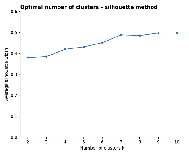
However, when applying the silhouette coefficient, a metric widely used in cluster analysis to analyze cluster quality [24], a maximum value was observed at 7 groups, with an average score of approximately 0.49. This metric considers not only the internal cohesion of each group, taking into account how close the elements are to one another within a cluster, but also the separation among clusters and how different they are from other groups, which makes it possible to estimate how well structured the total dataset is after the clustering process.
Automatic techniques for selecting k validate this decision and improve the initial segmentation, such as those proposed by the study [25], which use heuristic and mathematical strategies to refine the choice of the k parameter in K-Means [26].
These types of techniques prove effective because they avoid arbitrary or suboptimal decisions and make it possible to verify whether the number of groups determined by methods such as the elbow or silhouette method truly represents a meaningful structure in the data.
Figure 1. Clusters based on the elbow method
Figure 2. Cluster based on the silhouette method
With support from the silhouette-based coefficient and additional validation through automatic methods, it was possible to work with 7 clusters, as shown in Figure 2, since this offers a much clearer separation among network traffic patterns [27] and greater internal cohesion [28]. This configuration optimizes the model's ability to differentiate between normal and anomalous traffic types more precisely. The silhouette coefficient used in the research was calculated using mathematical Eq. (2):
$s(i)=\frac{b(i)-a(i)}{\max \{a(i), b(i)\}}$ (2)
The silhouette coefficient used in the research was calculated using mathematical Eq. (2). After selecting k = 7, the comparative application and evaluation of four clustering algorithms was performed. The K-Means model was applied to the complete post-PCA dataset, while the more computationally intensive methods (H-Clust, DBSCAN, CLARA) were applied to the random sample of 10,000 records (datos_muestra) to ensure the feasibility of the analysis. To ensure a fair, observation-matched comparison, K-Means was additionally re-fitted, using the same hyperparameters (centers = 7, nstart = 25), on the identical 10,000 record sample used for H-Clust, CLARA, and DBSCAN. This sample (datos_muestra) was drawn with a fixed random seed (set.seed(42)) to ensure reproducibility; its class distribution did not differ significantly from that of the complete dataset (χ² = 9.28, df = 9, p = 0.41). The baseline K-Means model was fitted on the complete dataset, while the model used for comparative evaluation was re-fitted on the shared sample. As a robustness check, we repeated the entire sampling-and-clustering pipeline with two additional seeds; the ranking among K-Means, H-Clust, and CLARA was not stable across seeds (Adjusted Rand Index (ARI) ranged approximately 0.08-0.13 for all three, with no method consistently ahead), whereas DBSCAN consistently obtained a near-zero ARI regardless of seed. This behavior directly informs how the comparative results should be interpreted.
Model 1: K-Means (Baseline)
The K-means algorithm was applied using 7 initial centers (centers = 7) and 25 random restarts (nstart = 25) on the complete principal component matrix (PCA). The use of multiple initializations seeks to avoid suboptimal local solutions, as has been validated in studies on high dimensional clustering.
Model 2: H-Clust
Hierarchical clustering was implemented using the hclust function on the Euclidean distance matrix of the sample (dist_muestra). The 'ward.D2' linkage method was selected, which minimizes total variance within the clusters and is conceptually similar to the objective of K-Means. Finally, the resulting dendrogram was cut at k = 7 to maintain comparability.
Model 3: CLARA
Given the large size of the dataset, the CLARA algorithm (CLARA function), an optimization of K-Medoids (PAM) designed for large volumes of data, was evaluated. It was configured to operate on the sample (sample_data), seeking 7 clusters (k = 7), using 50 subsamples (samples = 50) of 1,000 records each (sampsize = 1000) to determine the optimal medoids.
Model 4: DBSCAN
To explore anomaly detection and clusters with arbitrary shapes, DBSCAN (dbscan function) was used. Unlike the previous methods, DBSCAN does not require a k number of clusters. Its minPts and eps parameters were determined empirically. minPts was set at 80 (approximately 2 times the dimensionality of the original data, 2*40). The eps value (neighborhood radius) was estimated by visualizing the k-distance plot, selecting a value of 10, where an 'elbow' is observed (Figure 1). In this model, the points assigned to 'cluster 0' are considered noise or anomalies.
Comparative evaluation:
The quality of all models was evaluated externally by crossing the generated clusters with the real attack_cat label through contingency tables (purity). Additionally, internal silhouette metrics were analyzed for the partitional models (K-Means, H-Clust, CLARA), and the centroids or behaviors were interpreted.
3.1 Results of the K-Means model (Baseline)
After the initial cleaning of the UNSW-NB15 dataset, relevant numerical variables were selected for the unsupervised analysis. A transformation of the data was carried out through scaling, and then PCA was applied with the objective of reducing dimensionality and facilitating visualization of the clusters. First, the covariance matrix was calculated, as shown in Eq. (3).
$\Sigma=\frac{1}{n-1} X^T X$ (3)
Then, the eigenvectors v and eigenvalues λ were obtained by solving Eq. (4):
$\Sigma v=\lambda v$ (4)
Finally, the data are projected onto the first principal components, which in the case of the research were 10, and this was achieved through Eq. (5):
$Z=X W$ (5)
After dimensionality reduction with PCA, the 7 clusters were crossed with the attack_cat variable.
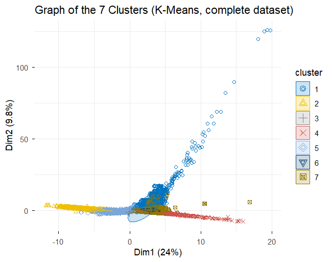
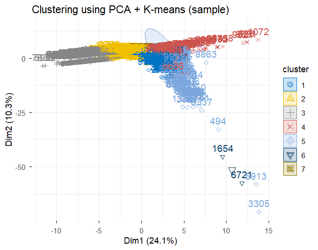
Table 1 shows that each cluster groups network flows with similar characteristics, evidencing patterns of normal or malicious traffic. Cluster 1 presents a 100% purity of legitimate (Normal) traffic, while Cluster 2 is highly specialized in Generic attacks (94.6%). In contrast, Clusters 3, 6, and 7 present a much more diverse composition, mixing attacks such as Exploits, DoS, Fuzzers, and Reconnaissance together with normal traffic. These results demonstrate K-Means' capacity to isolate specific high-purity behaviors, although it still struggles with complex separations in the densest regions of the dataset, as shown in Figure 3.
Table 1. K-Means cluster vs real attack categories
|
Cluster |
Analysis |
Backdoor |
DoS |
Exploits |
Fuzzers |
Generic |
Normal |
Reconnaissance |
Shellcode |
Worms |
|
1 |
0 |
0 |
0 |
0 |
0 |
0 |
914 |
0 |
0 |
0 |
|
2 |
0 |
0 |
0 |
0 |
91 |
9920 |
480 |
0 |
0 |
0 |
|
3 |
0 |
0 |
83 |
1078 |
1 |
112 |
11925 |
3 |
0 |
7 |
|
4 |
0 |
0 |
6 |
26 |
0 |
0 |
0 |
0 |
0 |
0 |
|
5 |
0 |
0 |
6 |
298 |
7 |
0 |
369 |
0 |
0 |
0 |
|
6 |
58 |
51 |
960 |
6352 |
3705 |
408 |
13899 |
1862 |
193 |
31 |
|
7 |
619 |
532 |
3034 |
3378 |
2258 |
8431 |
9413 |
1631 |
185 |
6 |
Figure 3. Graph of the 7 clusters
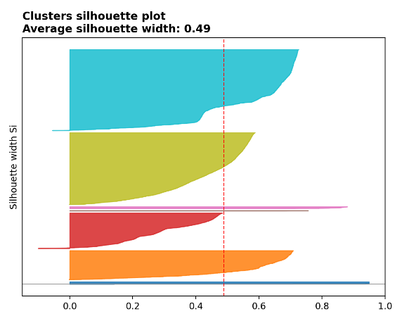
In Table 2, it can be seen that clusters 1 (0.89) and 5 (0.84) are well-defined clusters, since their silhouette widths approach 1, indicating strong internal cohesion and clear separation from other groups. Meanwhile, the weakest or least defined are clusters 3 (0.30) and 6 (0.43), which correspond precisely to the highly mixed and overlapping attack clusters identified in Table 1.
Table 2. Silhouette coefficient results by cluster
|
Cluster |
Size |
Average Silhouette Width |
|
|
1 |
109 |
0.89 |
|
|
2 |
1306 |
0.56 |
|
|
3 |
1600 |
0.30 |
|
|
4 |
7 |
0.63 |
|
|
5 |
77 |
0.84 |
|
|
6 |
3245 |
0.43 |
|
|
7 |
3656 |
0.58 |
|
|
Overall average: |
0.49 |
||
Note: Due to computational constraints for large matrices, Table 2 and Figure 4 are evaluated on the 10,000-record sample.
Figure 4 shows the quality of the clustering achieved through the clustering algorithm applied to the cybersecurity dataset, evidencing an average silhouette value of 0.49, which indicates moderate quality in the separation of the clusters. Although some groups, such as clusters 1, 4, and 5, present excellent internal cohesion and separation from the others, the largest groups (clusters 3, 6, and 7) possess much wider, overlapping profiles with lower individual silhouettes. Overall, this analysis suggests that while certain specific threats and normal behaviors can be cleanly isolated, the inherent complexity and overlap of cyberattack signatures make them difficult to partition perfectly with distance-based centroids.
k = 7 was retained, rather than the k = 3 suggested by the elbow method alone, because the silhouette coefficient (which, unlike WCSS, penalizes poor inter-cluster separation as well as poor intra-cluster cohesion) shows a marked improvement from k = 2 through k = 7 and then plateaus, with only marginal gains from additional clusters. We additionally retained k = 7 as a single, common configuration across all four algorithms specifically to preserve comparability in Section 3.2 to 3.4; we acknowledge this as a limitation, since three of the seven clusters remain small and weakly separated on the complete dataset.
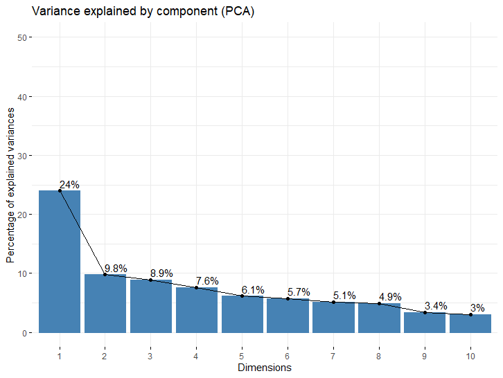
Figure 5 presents the scree plot of our PCA. Our methodological decision to retain the first 10 components (implemented in R as datos pca <- pca$x [1:10]) was based on the scree plot in Figure 5. As expected, variability is concentrated in the first dimensions, with the first component (PC1) explaining 24% and the second (PC2) 9.8% of the variance.
These ten components capture approximately 78% of the total variance (not approximately 50%, as an earlier draft of this section incorrectly stated, summing the individual variance percentages reported in Figure 5 gives 78.5%). Rather than assuming this level of retained variance reflects the intrinsic complexity of network traffic, we tested this empirically in Section 3.4 by comparing clustering quality across alternative variance-retention thresholds (70%, 80%, and 90%). Increasing the retained variance beyond 78% left the ARI essentially unchanged (0.104 at 10 components vs. 0.104 at 16 components) while reducing internal cohesion, indicating that additional components add limited discriminative value for this task.
Figure 4. Silhouette plot based on the principal component analysis (PCA) sample
Figure 5. Visualization of variance
3.2 Results of comparative models (on sample)
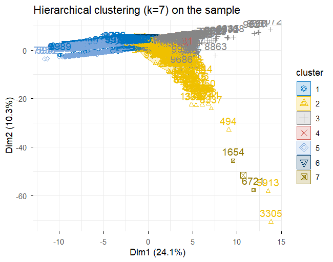
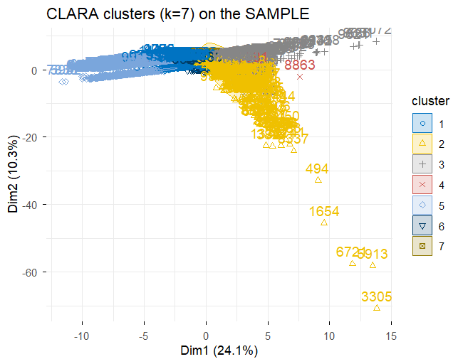
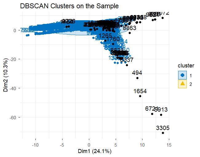
As illustrated in Figures 6-9, the spatial distribution of the generated clusters provides visual confirmation of the subsequent performance metrics. By projecting all four clustering solutions onto the identical two-dimensional PCA subspace (which captures 34.4% of the cumulative variance in its first two components), the structural behavior of each algorithm becomes directly comparable. K-Means (Figure 6), H-Clust (Figure 7), and CLARA (Figure 8) display geometrically distinct partitioning strategies, yet they all successfully divide the principal data mass into multiple identifiable regions. This visual segmentation corresponds directly to their statistically comparable, albeit modest, external validity (ARI ≈ 0.10). In sharp contrast, Figure 9 visually demonstrates the "DBSCAN paradox": rather than discovering meaningful density-based partitions within the network traffic, the algorithm collapses 99.0% of the observations into a single macro-cluster (Cluster 1, shown in blue), while merely isolating the most extreme spatial outliers (e.g., records 1654, 3305, and 6721) as noise. This visual evidence reinforces the empirical conclusion that centroid-, hierarchy-, and medoid-based approaches are better suited for this specific cybersecurity feature space than density-based methods.
Figure 6. Clusters with principal component analysis (PCA) + K-Means
Figure 7. Visualization of hierarchical agglomerative clustering (H-Clust) Clusters (k = 7) on the principal component analysis (PCA) sample
Figure 8. Visualization of Clustering Large Applications (CLARA) Clusters (k = 7) on the principal component analysis (PCA) sample
Figure 9. Visualization of Density-Based Spatial Clustering (DBSCAN) Clusters on the principal component analysis (PCA) sample
3.3 Description of model behavior by cluster
Table 3 shows that the combined use of PCA and K-Means on the UNSW-NB15 dataset made it possible to identify significant behavioral groupings in network traffic, with a segmentation that reflects an effective approximation to cyberthreat detection from an unsupervised perspective.
In Table 4, H-Clust identified and isolated several key network behaviors, closely matching the K-Means patterns given their comparable external validity. The model isolated a small group of brief, local-type sessions (Cluster 1), FTP login/command activity (Cluster 5), and a very small group of unusually large, lossy, long-duration sessions (Cluster 4). Download-type traffic with a heavy destination-side data load was captured in Cluster 2, while Clusters 3, 6, and 7, which together account for the majority of records, differ mainly in connection rate, TTL, and TCP round-trip time rather than in a single dominant behavior.
In Table 5, the analysis of the CLARA model shows a broadly similar structure to H-Clust and K-Means, but distributed somewhat more evenly across clusters. CLARA isolated brief, local-type sessions (Cluster 2) and download-type traffic with a heavy destination-side data load (Cluster 3), while Clusters 1 and 4 share a scanning-like signature of repeated connections to recent destinations at an elevated rate. Cluster 6 stands out for frequent HTTP method usage, consistent with web application traffic, and Clusters 5 and 7 differ mainly in TCP round-trip time, TTL, and connection-state consistency rather than in a single dominant behavior.
Table 3. Average description of behavior by principal component analysis (PCA) + K-Means cluster
|
Cluster |
Behavior Description |
|
1 |
Sessions with matching source/destination IP-port structure and short TTL, typical of brief local connections. |
|
2 |
Frequent repeated connections to the same service and destination at a high packet rate. |
|
3 |
Short-TTL sessions with a heavy destination-side data load, consistent with routine downloads. |
|
4 |
A very small group of unusually large, lossy, long-duration sessions. |
|
5 |
Sessions dominated by FTP login and command activity. |
|
6 |
Longer TCP round-trip times with low connection rate and little service repetition. |
|
7 |
High connection-state consistency and packet rate with short round-trip time. |
Table 4. Average description of behavior by hierarchical agglomerative clustering (H-Clust) cluster
|
Cluster |
Behavior Description |
|
1 |
Sessions with matching source/destination IP-port structure and short TTL, typical of brief local connections. |
|
2 |
Short-TTL sessions with heavy destination-side data load and an atypical connection-state pattern. |
|
3 |
Frequent repeated connections to the same service and destination with high connection-state consistency. |
|
4 |
A very small group of unusually large, lossy, long-duration sessions. |
|
5 |
Sessions dominated by FTP login and command activity. |
|
6 |
Longer TCP round-trip times with low connection rate and little service repetition. |
|
7 |
High packet rate and source-side data load with short round-trip time. |
Table 5. Average description of behavior by Clustering Large Applications (CLARA) cluster
|
Cluster |
Behavior Description |
|
1 |
Frequent repeated connections to the same service and destination at a high packet rate. |
|
2 |
Short-TTL sessions with matching source/destination IP-port structure, typical of brief local connections. |
|
3 |
Short-TTL sessions with a heavy destination-side data load, consistent with routine downloads. |
|
4 |
Repeated service connections to recent destinations at an elevated packet rate. |
|
5 |
Longer TCP round-trip times with low connection rate and little service repetition. |
|
6 |
Frequent HTTP method usage with short TTL, consistent with web application traffic. |
|
7 |
High TTL and connection-state consistency with an elevated packet rate. |
In Table 6, DBSCAN's behavior sheds light on its grouping logic. With the parameters used here, the algorithm aggregated 99.0% of the sample into a single 'macro-cluster' (Cluster 1) whose feature averages sit close to the overall dataset mean, indicating an absence of meaningful internal differentiation, consistent with the near-zero ARI. The points assigned to noise (Cluster 0, 98 records, 0.98% of the sample) are not random: they are characterized by elevated FTP login/command activity and substantial packet loss, suggesting DBSCAN isolates a narrow band of technically unusual FTP sessions as outliers rather than identifying broader threat categories.
Table 6. Average description of behavior by Density-Based Spatial Clustering (DBSCAN) cluster
|
Cluster |
Behavior Description |
|
0 |
Noise points dominated by FTP login/command activity and packet loss, distinct from the main traffic mass. |
|
1 |
A single macro-cluster whose feature averages sit close to the overall dataset mean, reflecting DBSCAN's inability to differentiate sub-structure within the main traffic mass. |
The analysis of Table 7 (unified contingency table) allows a direct comparison of each model's cluster assignment against the real attack categories. The K-Means and H-Clust sections show closely similar structures, consistent with their comparable ARI: both isolate a small, fully 'Normal' cluster (109 and 103 records, respectively) and a high-purity 'Generic' cluster (K-Means Cluster 2, 1,234/1,314 records; H-Clust Cluster 3, 1,278/1,380 records), while their largest clusters remain heterogeneous, mixing 'Exploits', 'Fuzzers', 'Generic', and 'Normal' traffic (K-Means Cluster 7: 3,648 records, 1,175 'Normal' and 999 'Generic'; H-Clust Cluster 7: 3,582 records, 1,155 'Normal' and 955 'Generic'). The CLARA section presents a broadly similar pattern but distributes records more evenly across clusters: it isolates a fully 'Generic' cluster (Cluster 1, 408 records) and two high-purity 'Normal' clusters (Clusters 2 and 3, above 90% 'Normal'), while Clusters 5-7 mix 'Exploits', 'DoS', and 'Fuzzers' with 'Normal' and 'Generic' traffic. Finally, the DBSCAN section confirms the pattern already visible in Table 8: Cluster 1 (9,902 records, 99.0% of the sample) mixes all traffic types (4,459 'Normal', 2,296 'Generic', 1,291 'Exploits', 734 'Fuzzers', 515 'DoS'), and even the 98 records assigned to noise (Cluster 0) are themselves a mixture (53 'Normal', 40 'Exploits'), confirming that DBSCAN, with the parameters used here, does not partition attack categories in any interpretable way.
Table 7. Detailed analysis of the contingency tables
|
Model |
Cluster |
Analysis |
Backdoor |
DoS |
Exploits |
Fuzzers |
Generic |
Normal |
Reconnaissance |
Shellcode |
Worms |
|
K-Means |
1 |
0 |
0 |
0 |
0 |
0 |
0 |
109 |
0 |
0 |
0 |
|
K-Means |
2 |
0 |
0 |
0 |
0 |
11 |
1234 |
69 |
0 |
0 |
0 |
|
K-Means |
3 |
0 |
0 |
9 |
135 |
0 |
13 |
1442 |
1 |
0 |
1 |
|
K-Means |
4 |
0 |
0 |
2 |
5 |
0 |
0 |
0 |
0 |
0 |
0 |
|
K-Means |
5 |
0 |
0 |
0 |
33 |
0 |
0 |
44 |
0 |
0 |
0 |
|
K-Means |
6 |
8 |
8 |
110 |
737 |
447 |
51 |
1673 |
189 |
17 |
4 |
|
K-Means |
7 |
91 |
67 |
397 |
421 |
277 |
999 |
1175 |
198 |
22 |
1 |
|
H-Clust |
1 |
0 |
0 |
0 |
0 |
0 |
0 |
103 |
0 |
0 |
0 |
|
H-Clust |
2 |
0 |
0 |
3 |
23 |
0 |
5 |
1278 |
0 |
0 |
1 |
|
H-Clust |
3 |
2 |
1 |
1 |
2 |
6 |
1278 |
89 |
1 |
0 |
0 |
|
H-Clust |
4 |
0 |
0 |
2 |
5 |
0 |
0 |
0 |
0 |
0 |
0 |
|
H-Clust |
5 |
0 |
0 |
0 |
33 |
0 |
0 |
44 |
0 |
0 |
0 |
|
H-Clust |
6 |
8 |
8 |
116 |
849 |
447 |
59 |
1843 |
190 |
17 |
4 |
|
H-Clust |
7 |
89 |
66 |
396 |
419 |
282 |
955 |
1155 |
197 |
22 |
1 |
|
CLARA |
1 |
0 |
0 |
0 |
0 |
0 |
408 |
0 |
0 |
0 |
0 |
|
CLARA |
2 |
0 |
0 |
13 |
10 |
1 |
2 |
770 |
0 |
0 |
0 |
|
CLARA |
3 |
0 |
0 |
5 |
97 |
0 |
7 |
1271 |
0 |
0 |
0 |
|
CLARA |
4 |
2 |
1 |
1 |
2 |
23 |
879 |
101 |
1 |
0 |
0 |
|
CLARA |
5 |
8 |
7 |
66 |
526 |
432 |
34 |
1405 |
157 |
17 |
2 |
|
CLARA |
6 |
0 |
1 |
50 |
287 |
14 |
23 |
442 |
33 |
0 |
3 |
|
CLARA |
7 |
89 |
66 |
383 |
409 |
265 |
944 |
523 |
197 |
22 |
1 |
|
DBSCAN |
0 |
0 |
0 |
3 |
40 |
1 |
1 |
53 |
0 |
0 |
0 |
|
DBSCAN |
1 |
99 |
75 |
515 |
1291 |
734 |
2296 |
4459 |
388 |
39 |
6 |
Note: hierarchical agglomerative clustering (H-Clust), Clustering Large Applications (CLARA), Density-Based Spatial Clustering (DBSCAN).
The analysis of Table 8 shows that K-Means, H-Clust (Ward.D2), and CLARA achieve statistically comparable external validity: their ARI values (0.103, 0.104, and 0.101, respectively) differ by less than the variation observed when the sampling procedure is repeated with different random seeds (ARI ranging approximately 0.08-0.13 across seeds), so we do not consider any single one of these three methods to be robustly superior on this dataset. CLARA achieved the highest Purity (0.612) and Rand Index (0.668) of the three, while H-Clust achieved the lowest Davies-Bouldin Score (0.659), indicating a marginally more compact and better-separated internal structure; none of these differences, however, was large or stable enough across seeds to support a claim of overall superiority. DBSCAN, in clear contrast, obtained the lowest Purity (0.451) and a near-zero ARI (−0.001), consistently across every seed tested.
Table 8. Performance evaluation of the evaluation methods
|
Model |
P |
RI |
ARI |
SS |
DBS |
|
K-Means |
0.5682 |
0.6362696 |
0.102830016 |
0.4881274 |
0.650028 |
|
H-Clust |
0.5706 |
0.6334588 |
0.104187208 |
0.4715285 |
0.658551 |
|
CLARA |
0.6119 |
0.6675123 |
0.100855414 |
0.3752932 |
1.215239 |
|
DBSCAN |
0.4512 |
0.2914553 |
-0.000971695 |
0.7711664 |
1.516938 |
Note: P = Purity; RI = Rand Index; ARI = Adjusted Rand Index; SS = Silhouette Score; DBS = Davies-Bouldin Score; H-Clust = hierarchical agglomerative clustering; CLARA = Clustering Large Applications; DBSCAN = Density-Based Spatial Clustering.
The most striking finding of this comparison remains the DBSCAN paradox. This model obtained the best internal scores when noise points are counted as their own group (Silhouette of 0.771 and DBS of 1.517), but its ARI was near zero (−0.001) and its Purity the lowest of the four models (0.451). Once noise points are excluded entirely, only a single real cluster remains, so internal separation metrics become undefined; the apparently strong internal score is therefore an artifact of treating noise as a legitimate cluster, not evidence of meaningful structure. This shows that, although DBSCAN's parameters produced a geometrically compact grouping, it has no positive correlation with the real attack categories and performed worse than random grouping, so we consider it the least suitable of the four models for this problem.
3.4 Sensitivity analysis of principal component analysis dimensionality
To empirically test whether retaining ten principal components (≈78% of the total variance) discards attack-relevant information, K-Means (centers = 7, nstart = 25) was re-fitted on the complete dataset using the number of components required to reach 70%, 80%, and 90% cumulative explained variance, in addition to the original ten. For each configuration we report the ARI against the true attack_cat labels and the average silhouette width (evaluated on the fixed 10,000 record sample described in Section 2).
The ARI is essentially unchanged across this range (0.104 throughout, to three decimal places), while the average silhouette declines steadily as more components are added. This indicates that components beyond the original ten add limited discriminative value for separating the true attack categories, even though they continue to explain additional variance; retaining ten components therefore reflects a reasonable, empirically supported trade-off between dimensionality reduction and information loss for this clustering task, rather than an assumption asserted a priori (Table 9).
Table 9. Sensitivity analysis of principal component analysis (PCA) dimensionality
|
Components |
Cum. Variance |
Avg. Silhouette |
ARI |
|
8 (≥70%) |
72.05% |
0.547 |
0.104 |
|
10 (original, ≥78%) |
78.43% |
0.488 |
0.104 |
|
11 (≥80%) |
81.09% |
0.471 |
0.104 |
|
16 (≥90%) |
90.56% |
0.432 |
0.104 |
When evaluating the performance of the PCA and clustering pipeline on the UNSW-NB15 dataset, it becomes clear that threat detection is not only a grouping challenge [29], but also a challenge of interpreting latent structures in traffic [30]. A methodologically important point is that retaining 10 principal components explains approximately 78% of the total variance, not approximately 50% as an earlier draft of this manuscript stated; the sensitivity analysis in Section 3.4 shows that this level of retained variance is empirically sufficient, since additional components leave external validity (ARI) unchanged while only reducing internal cohesion, consistent with the behavioral entropy of modern traffic [31]. The nature of current cyberattacks is so mixed with legitimate traffic that linear projections usually require deep multidimensional analysis to avoid the loss of critical signals [32], even when compared with modern autoencoder techniques [33].
The comparable performance of K-Means, H-Clust (Ward.D2), and CLARA (ARI between approximately 0.10 and 0.13, depending on the random seed) suggests that, for this dataset, network traffic does not clearly favor one partitioning geometry over another: centroid based, hierarchical, and medoid based methods all recover a similarly modest amount of the structure defined by the ground truth attack categories. This instability across seeds is itself an important finding, and directly motivated our decision to fix and report a random seed and to test multiple seeds as a robustness check. This behavior validates the thesis of Rehman [34], who argue that models that respect local density are the only ones capable of adapting to the heterogeneity of anomalies in dynamic network environments [35]. A finding that breaks with conventional logic is the "DBSCAN Paradox" [36].
Despite obtaining an excellent internal silhouette (0.771), its negative ARI (-0.001) reveals that it created mathematically compact groups but ones lacking semantic meaning, collapsing 99.00% of the traffic into a single amorphous mass. As Bhattacharjee and Mitra warn, after dimensionality reduction with PCA, traffic density can become so uniform that it prevents DBSCAN from distinguishing clear boundaries between normal and malicious activities [37].
The results show that, once a fixed and documented random sample is used, K-Means, hierarchical clustering (Ward.D2), and CLARA achieve comparable, moderate alignment with the true attack categories in the UNSW-NB15 dataset (ARI approximately 0.10-0.13 depending on the random seed), with no single method consistently and robustly outperforming the others. DBSCAN, by contrast, consistently fails to meaningfully partition network traffic under the tested parameters, regardless of the sampling seed.
PCA remains an indispensable component for the computational feasibility of the pipeline, retaining approximately 78% of the total variance in ten components; our sensitivity analysis (Section 3.4) shows that additional components yield no meaningful gain in external validity. However, PCA's dimensionality reduction appears to homogenize local data density in a way that limits DBSCAN's ability to distinguish meaningful boundaries, consistent with the “DBSCAN paradox” observed in Section 4.
This underscores that model evaluation cannot rely on internal cohesion metrics such as the Silhouette index alone, but must incorporate external, label-based validation such as the ARI.
Overall, the findings suggest that unsupervised clustering pipelines for cybersecurity should report a fixed, documented random seed and, where feasible, test robustness across multiple seeds, since the specific ranking among partition-based methods can otherwise be unstable even though the qualitative conclusion, that density-based clustering underperforms on this task, remains robust. Future research should explore federated learning and swarm-intelligence-based hyperparameter optimization, as well as testing this pipeline on additional intrusion-detection benchmarks, to strengthen the resilience and generalizability of unsupervised detection systems.
The UNSW-NB15 dataset analyzed in this study is publicly available from the UNSW Canberra Cyber Range Lab at https://research.unsw.edu.au/projects/unsw-nb15-dataset and is described by Moustafa and Slay. No new empirical data were generated for this study. The cleaned dataset, PCA scores, cluster assignments, and analysis scripts produced during this revision are available from the corresponding author upon reasonable request.
To improve the linguistic quality and clarity of this manuscript, the authors used an AI-based language tool.
The AI tool was not used to generate, analyze, or determine the fundamental scientific content of this work. Consequently, the authors retain full responsibility for the information presented in this manuscript.
[1] García-Teodoro, P., Díaz-Verdejo, J., Maciá-Fernández, G., Vázquez, E. (2009). Anomaly-based network intrusion detection: Techniques, systems and challenges. Computers & Security, 28(1-2): 18-28. https://doi.org/10.1016/j.cose.2008.08.003
[2] Sommer, R., Paxson, V. (2010). Outside the closed world: On using machine learning for network intrusion detection. In 2010 IEEE Symposium on Security and Privacy, pp. 305-316. https://doi.org/10.1109/SP.2010.25
[3] Chandola, V., Banerjee, A., Kumar, V. (2009). Anomaly detection: A survey. ACM Computing Surveys, 41(3): 1-58. https://doi.org/10.1145/1541880.1541882
[4] Thaseen, I.S., Kumar, C.A. (2014). Intrusion detection model using fusion of PCA and optimized SVM. In 2014 International Conference on Contemporary Computing and Informatics (IC3I), Mysore, India, pp. 879-884. https://doi.org/10.1109/IC3I.2014.7019692
[5] Sadegh-Zadeh, S.A., Tajdini, M. (2025). An unsupervised machine learning approach for cyber threat detection using geographic profiling and Domain Name System data. Decision Analytics Journal, 15: 100576. https://doi.org/10.1016/j.dajour.2025.100576
[6] Fernandez Maimo, L., Perales Gomez, A.L., Garcia Clemente, F.J., Gil Perez, M., Martinez Perez, G. (2018). A self-adaptive deep learning-based system for anomaly detection in 5G networks. IEEE Access, 6: 7700-7712. https://doi.org/10.1109/ACCESS.2018.2803446
[7] Wang, Y.X. (2024). Deep learning-based network intrusion detection systems. Applied and Computational Engineering, 109(1): 179-188. https://doi.org/10.54254/2755-2721/2024.18104
[8] Jaradat, A.S., Barhoush, M.M., Bani Easa, R.S. (2022). Network intrusion detection system: Machine learning approach. Indonesian Journal of Electrical Engineering and Computer Science, 25(2): 1151-1158. https://doi.org/10.11591/ijeecs.v25.i2.pp1151-1158
[9] Kaliyaperumal, P., Periyasamy, S., Thirumalaisamy, M., Balusamy, B., Benedetto, F. (2024). A novel hybrid unsupervised learning approach for enhanced cybersecurity in the IoT. Future Internet, 16(7): 253. https://doi.org/10.3390/fi16070253
[10] Pajouh, H.H., Javidan, R., Khayami, R., Dehghantanha, A., Choo, K.K.R. (2019). A two-layer dimension reduction and two-tier classification model for anomaly-based intrusion detection in IoT backbone networks. IEEE Transactions on Emerging Topics in Computing, 7(2): 314-323. https://doi.org/10.1109/TETC.2016.2633228
[11] Moustafa, N., Slay, J. (2015). UNSW-NB15: A comprehensive data set for network intrusion detection systems (UNSW-NB15 network data set). In 2015 Military Communications and Information Systems Conference (MilCIS), Canberra, ACT, Australia, pp. 1-6. https://doi.org/10.1109/MilCIS.2015.7348942
[12] Yuan, S.H., Wu, X.T. (2021). Deep learning for insider threat detection: Review, challenges and opportunities. Computers & Security, 104: 102221. https://doi.org/10.1016/j.cose.2021.102221
[13] Shiravi, A., Shiravi, H., Tavallaee, M., Ghorbani, A.A. (2012). Toward developing a systematic approach to generate benchmark datasets for intrusion detection. Computers & Security, 31(3): 357-374. https://doi.org/10.1016/j.cose.2011.12.012
[14] Muniyandi, A.P., Rajeswari, R., Rajaram, R. (2012). Network anomaly detection by cascading K-Means clustering and C4.5 decision tree algorithm. Procedia Engineering, 30: 174-182. https://doi.org/10.1016/j.proeng.2012.01.849
[15] Liu, F.T., Ting, K.M., Zhou, Z.H. (2008). Isolation forest. In 2008 Eighth IEEE International Conference on Data Mining, Pisa, Italy, pp. 413-422. https://doi.org/10.1109/ICDM.2008.17
[16] Breunig, M.M., Kriegel, H.P., Ng, R.T., Sander, J. (2000). LOF: Identifying density-based local outliers. ACM SIGMOD Record, 29(2): 93-104. https://doi.org/10.1145/335191.335388
[17] Zimek, A., Filzmoser, P. (2018). There and back again: Outlier detection between statistical reasoning and data mining algorithms. WIREs Data Mining and Knowledge Discovery, 8(6): e1280. https://doi.org/10.1002/widm.1280
[18] Jolliffe, I.T., Cadima, J. (2016). Principal component analysis: A review and recent developments. Philosophical Transactions of the Royal Society A: Mathematical, Physical and Engineering Sciences, 374(2065): 20150202. https://doi.org/10.1098/rsta.2015.0202
[19] Jolliffe, I.T. (2002). Principal Component Analysis (2nd ed.). Springer Series in Statistics. New York: Springer-Verlag. https://doi.org/10.1007/b98835
[20] Jain, A.K. (2010). Data clustering: 50 years beyond K-means. Pattern Recognition Letters, 31(8): 651-666. https://doi.org/10.1016/j.patrec.2009.09.011
[21] Saxena, A., Prasad, M., Gupta, A., et al. (2017). A review of clustering techniques and developments. Neurocomputing, 267: 664-681. https://doi.org/10.1016/j.neucom.2017.06.053
[22] Santoso, N.A., Lutfayza, R., Nughroho, B.I., Gunawan, G. (2024). Anomaly detection in network security systems using machine learning. Journal of Intelligent Decision Support System (IDSS), 7(2): 113-120. https://doi.org/10.35335/idss.v7i2.238
[23] Erfani, S.M., Rajasegarar, S., Karunasekera, S., Leckie, C. (2016). High-dimensional and large-scale anomaly detection using a linear one-class SVM with deep learning. Pattern Recognition, 58: 121-134. https://doi.org/10.1016/j.patcog.2016.03.028
[24] Rousseeuw, P.J. (1987). Silhouettes: A graphical aid to the interpretation and validation of cluster analysis. Journal of Computational and Applied Mathematics, 20: 53-65. https://doi.org/10.1016/0377-0427(87)90125-7
[25] Kilincer, I.F., Ertam, F., Sengur, A. (2021). Machine learning methods for cyber security intrusion detection: Datasets and comparative study. Computer Networks, 188: 107840. https://doi.org/10.1016/j.comnet.2021.107840
[26] Anthi, E., Williams, L., Javed, A., Burnap, P. (2021). Hardening machine learning denial of service (DoS) defences against adversarial attacks in IoT smart home networks. Computers & Security, 108: 102352. https://doi.org/10.1016/j.cose.2021.102352
[27] Kasongo, S.M., Sun, Y.X. (2020). A deep learning method with wrapper based feature extraction for wireless intrusion detection system. Computers & Security, 92: 101752. https://doi.org/10.1016/j.cose.2020.101752
[28] Kumar, L.K.S., Nethi, S.R., Uyyala, R., et al. (2026). Anomaly-based intrusion detection on benchmark datasets for network security: A comprehensive evaluation. Scientific Reports, 16(1): 8507. https://doi.org/10.1038/s41598-026-38317-w
[29] Kayode Saheed, Y., Idris Abiodun, A., Misra, S., Kristiansen Holone, M., Colomo-Palacios, R. (2022). A machine learning-based intrusion detection for detecting internet of things network attacks. Alexandria Engineering Journal, 61(12): 9395-9409. https://doi.org/10.1016/j.aej.2022.02.063
[30] Kumar, V., Das, A.K., Sinha, D. (2020). Statistical analysis of the UNSW-NB15 dataset for intrusion detection. In Security and Communication Networks, Springer, Singapore, pp. 279-294. https://doi.org/10.1007/978-981-13-9042-5_24
[31] Tory, A.R., Hasan, K.F. (2026). An evaluation framework for network IDS/IPS datasets: Leveraging MITRE ATT&CK and industry relevance metrics. Computers & Security, 161: 104777. https://doi.org/10.1016/j.cose.2025.104777
[32] Pamena, A., Sugali, M.N. (2025). SAE-AM: Enhancing network intrusion detection using sparse autoencoders with attention modules. Applied Cybersecurity & Internet Governance, 4(1): 234-271. https://doi.org/10.60097/ACIG/213872
[33] Obeidat, M., Shehab, R. (2025). Network-based intrusion detection in IoT environments using hybrid machine learning techniques. Babylonian Journal of Networking, 2025: 116-125. https://doi.org/10.58496/BJN/2025/010
[34] Rehman, M., Kalakoti, R., Bahşi, H. (2025). Comprehensive feature selection for machine learning-based intrusion detection in healthcare IoMT networks. In Proceedings of the 11th International Conference on Information Systems Security and Privacy, SCITEPRESS-Science and Technology Publications, pp. 248-259. https://doi.org/10.5220/0013313600003899
[35] Mudgal, P. (2026). Clustering of temporal and visual data: Recent advancements. Data, 11(1): 7. https://doi.org/10.3390/data11010007
[36] Monshizadeh, M., Khatri, V., Kantola, R., Yan, Z. (2022). A deep density based and self-determining clustering approach to label unknown traffic. Journal of Network and Computer Applications, 207: 103513. https://doi.org/10.1016/j.jnca.2022.103513
[37] Bhattacharjee, P., Mitra, P. (2021). A survey of density based clustering algorithms. Frontiers of Computer Science, 15(1): 151308. https://doi.org/10.1007/s11704-019-9059-3