Natthaphong Luangnaruedom*![]() | Somchai Prakancharoen
| Somchai Prakancharoen![]() | Thavatchai Ngamsantivong
| Thavatchai Ngamsantivong![]()
© 2025 The authors. This article is published by IIETA and is licensed under the CC BY 4.0 license (http://creativecommons.org/licenses/by/4.0/).
OPEN ACCESS
The research aims to develop a preliminary solution for detecting database manipulation and identifying security risks. The experimental sample was implemented in a small enterprise in Thailand. Three users’ database manipulation logs were collected for six days and twelve hours of work per day in a week. The gathered data was used to seek the sequential patterns of their SQL commands using GSP sequential pattern analysis. The Markov chain is derived from the users' database manipulation sequence transactions and the identified sequential patterns. The undesirable incidents that occurred on that day were recorded in the logs. The occurrence of undesirable incidents on a single day of the week was calculated from the whole database manipulation sequence transactions. The hidden Markov chain is illustrated by the combination of undesirable incidents occurring on a single day of the week and effective items, along with their probabilities. The probability and the path of items that caused the undesirable incident were presented. Therefore, a database administrator could create a rule to prevent the possible occurrence of an unpleasant incident. This database manipulation security risk detection preliminary solution was validated through testing, achieving a 73.68% accuracy detection. After three months of implementing proactive prevention and adaptation, the proposed security protocol can reduce the mean time to repair (MTTR) by approximately seventy-five percent. Moreover, the mean time before failure (MTBF) is expanded from twenty hours to seventy-one hours. Therefore, the proposed security protocol could help DBAs prevent database manipulation failures by combining SQL commands.
database security protocol, GSP algorithm, Markov chain
The leading cause of this research comes from the organization’s database manipulation problems. The experimental case study is a small enterprise operation in Thailand. The sample organization is a domestic merchandising company specializing in agricultural products. There are only three IT users who are responsible for manipulating the organization’s database via application programs and directly using SQL commands. The research limitation is on the most essential organizational database that supports many users’ applications. The experience and digital competency of these IT users in database management systems are at a low to medium scale. These conditions could cause undesirable incidents in the organization’s database manipulation. Some undesirable incidents could cause faults or even failures in the organization’s data processing. The company sometimes works slowly or stops working altogether. This is why organizations must find a solution to the database manipulation security risk. Undesirable incidents could occur when many SQL statements are executed simultaneously. The research aims to see patterns of concurrent working SQL statements that could cause undesirable incidents. These patterns will be used to detect or monitor whether the damage is likely to occur or not. Many computer departments aim to educate their IT users about the dangers of using individual SQL commands so that undesirable incidents do not occur and cause database system manipulation failure. However, many database system faults and failures occurred from a combination of non-dangerous SQL commands being processed. The study of simultaneous processing command patterns that cause database faults will help DBAs focus on preventing database manipulation failures.
1.1 Objective
A) Create a preliminary database manipulation security risk detection solution.
B) Evaluate the accuracy of the security risk detection protocol.
C) Evaluate the database manipulation mean time to repair (MTTR) reduction of the proposed protocol. The percentage of MTTR should be reduced by at least fifty percent.
1.2 Advantage
The research contribution to the proposed preliminary database manipulation security risk detection solution creation could benefit organizational information system operations in two ways.
A) The organization’s data processing is stable, working on database manipulation.
B) The department’s maintenance time or system recovery cost is decreased.
2.1 SQL command
The experimental sample organization database manipulation commands are limited to the most commonly used MySQL commands in organizational applications. Sometimes, organizational DB users have to use SQL commands to manage their work directly. Many SQL commands support database operations. This research will consider covering only the fundamental, commonly used SQL commands, such as CREATE, INSERT, SELECT, UPDATE, DELETE, and GRANT [1].
2.2 Risk type, source of cause, damage mitigation
Some SQL commands can cause undesirable incidents when used individually. Nevertheless, the combination of SQL commands that are simultaneously running can cause some damage incidents [2]. Table 1 presents the risk type, an example of a dangerous command, and a suggested solution to reduce the damage caused by some dangerous SQL commands.
Table 1. SQL command risk management
|
SQL Command |
Risk Type |
Example of a Dangerous Statement |
Solution to Mitigate the Risk of Undesirable Incident |
|
CREATE |
- |
- |
- |
|
GRANT |
Privilege Escalation |
GRANT SELECT ON DATABASE:AbcDatabase TO John; |
Role based access control (most dangerous statements) |
|
INSERT |
Inject false records or manipulate data lineage, data inconsistencies. |
INSERT INTO destination table SELECT column1, column2, ... FROM source table WHERE condition; |
Apply input validation, restrict INSERT permission based on role |
|
UPDATE |
Modify sensitive data (Integrity loss) Data tampering |
UPDATE Customers SET ContactName='John'; |
Approval flow, audit logs, If you omit the WHERE clause, ALL records will be updated! |
|
DELETE |
Data loss, sabotage, removal of all the table's records |
DELETE FROM interactions; |
Provide soft deleting, detect of where clause omitting |
|
SELECT |
Mass data extraction |
-SELECT * -SELECT UserId, Name, Password FROM Users WHERE UserId = 999 or 1=1 |
Use SQL Parameters for Protection |
2.3 GSP and research practical example
A) GSP algorithm
The GSP algorithm (Generalized Sequential Pattern algorithm) [3-5] is frequently used for sequence mining in data mining. The algorithms for solving sequence mining problems are based on the Apriori (level-wise) algorithm. The generalized sequential pattern algorithm (GSP), based on a level-wise or a priori algorithm, is primarily used to discover the pattern of sequential items whose order of occurrence is essential. Data mining uses GSP to identify sequential behavior patterns. Patterns of insights appear in various applications, such as customer behavior when purchasing products. The plain data from the historical transactions (database) of all users, such as customers, regarding their purchased items on some date, are used to prepare the details of the customer sequence item purchasing transaction. These sequences will be counted to determine the support or number of each item occurring in all customer sequence item transactions. The support criteria are defined by the person responsible for data analytics. If the support number is enormous, then there will be a few candidate nodes that pass the support criteria. If the support number is minimal, many candidate nodes will be obtained. The maximum number of supports is the total number of sequence transactions. The other criterion of sequential pattern analysis is the confidence number. This criterion is not considered for all transaction numbers as support numbers, but only for those where the specified item is present. This research chose to omit the confidence criteria since the large number of item nodes could give a comprehensive picture of item node connections. All prepared candidate item nodes begin with one, two, three, or n candidate item nodes. If there is no matched support in the support criteria of any candidate item node from all sequence transactions, the number of candidate item nodes (n) will be set to 0.
The Apriori algorithm is commonly used to identify patterns of an item that emerge when a particular item occurs. The related item pattern is regardless of time. The number of each item is also ignored. The temporal data about SQL commands used is very important for detecting the IT user’s SQL command usage behavior. GSP [6, 7] solves these limitations by separating on an adjacent timescale. Moreover, the number of occurring items should be tagged with a finite number of powers, such as An.
Many algorithms utilize the Apriori algorithm to generate sequential patterns, such as GSP, and Sequential Pattern Discovery using Equivalence classes (SPADE) [8, 9]. The GSP algorithm is suitable for small datasets and short item sequences. Sometimes, GSP generates a repetitive candidate pattern. It is less complex and uses more calculation time. However, GSP should project all possible candidate sequences so that all possible sequence patterns will be gathered. The SPADE algorithm is used to create a sequence of patterns from a group of sequential transactions that use equivalent classes. GSP is not suitable for dense datasets in some classes, while other classes have sparse data. Other sequential pattern analyses, such as Prefix-projected Sequential Pattern Mining (PrefixSpan) and FreeSpan. The PrefixSpan uses a divide-and-conquer technique to separate subsequences and identify frequent patterns. This technique is suitable for large datasets and long-sequence transactions and is more complex.
Table 2. The user sequence of states is sorted by transaction date
|
Transaction Date |
User-ID |
State |
State Sequence (Date) |
||||
|
|
|
|
SID |
1 |
2 |
3 |
4 |
|
1 |
1 |
A |
1 |
<A, |
B, |
(AB), |
C> |
|
2 |
1 |
B |
|
|
|
|
|
|
3 |
1 |
(AB) |
|
|
|
|
|
|
4 |
1 |
C |
|
|
|
|
|
|
1 |
2 |
B |
2 |
<B, |
B, |
A, |
C> |
|
2 |
2 |
B |
|
|
|
|
|
|
3 |
2 |
A |
|
|
|
|
|
|
4 |
2 |
C |
|
|
|
|
|
|
1 |
3 |
(AB) |
3 |
<(AB), |
B |
B |
B> |
|
2 |
3 |
B |
|
|
|
|
|
|
3 |
3 |
B |
|
|
|
|
|
|
4 |
3 |
B |
|
|
|
|
|
B) GSP practical example
For example, consider the simple transaction data of three users (user IDs 1, 2, and 3) across three states of participation (A, B, and C). The user’s states were collected over four days. The data preparation is the first step of the GSP algorithm. The details of each user’s state participation are presented in Table 2.
Since joining the system, User ID-1 has had four transactions. He has chosen states ‘A’, ‘B’, ‘(AB)’, and ‘C’ for transaction dates #1, 2, 3, and 4, respectively. A single state indicates that this state is chosen on that day; for example, ‘A’. The symbol ‘(AB)’ suggests that states A and B are selected on the same transaction date. The state sequence of user ID 1 is. The order of the items (separated by ‘,’) shows which items occurred before. For example, ‘B’ states or is chosen after item ‘A’. The explanation above is the first step of the GSP activity, data preparation. The GSP algorithm's second step is to define the support criteria for GSP. In this example, the support number is given on number three, ‘3’. In step three, the number of each single-occurring state or item is counted from Table 2. The number of all occurring items is present in Table 3.
Table 3. The total count of each 1-item from all states or item sequences (Table 2)
|
-1-Item |
Support Count |
Pass-p |
|
A |
3 |
p |
|
B |
3 |
p |
|
C |
2 |
F |
Item ‘A’ appears in SID #1, 2, and 3, even though ‘A’ is present four times. However, the support number of ‘A’ will be calculated based on the number of states or item sequences, which have a maximum of three transaction SIDs. The item ‘C’ has a lower support number (2), so the one-item node ‘C’ is purged from further sequential pattern analysis. The fourth step is to create all the possible 2-item candidate nodes. Tables 4 and 5 show all possible two-item node patterns.
Table 4. The possible two-item node patterns on before and after positions
|
-2-Item |
A |
B |
C |
|
A |
A,A |
A,B |
A,C |
|
B |
B,A |
B,B |
B,C |
|
C |
C,A |
C,B |
C,C |
In the two-item node in Table 4, the first item precedes the second item. For example, ‘A, B’, item ‘A’ occurs on the transaction date (e.g., ‘t’), and ‘B’ appears on the following transaction date (e.g., ‘t+1’). The two-item node in Table 5 indicates that the first and second items co-occur. Thus, the sequence or position of the item is insignificant, and ‘(AB)’ = ‘(BA)’.
Table 5. The possible two-item node patterns occurred at the same time
|
A |
B |
C |
|
|
A |
(AA) |
(AB) |
(AC) |
|
B |
|
(BB) |
(BC) |
|
C |
|
|
(CC) |
These fifteen two-item candidate nodes are counted for each candidate node support. The results of the counting are presented in Table 6. There are only three two-item nodes, ‘AB’, ‘BB’, and (AB), that can pass the support number criteria. These nodes will be used to generate a three-item candidate node in the fifth step.
Table 6. The possible two-item node with support number results
|
-2-Item Node |
Support |
Pass-p |
|
AA |
2 |
|
|
AB |
3 |
p |
|
AC |
2 |
|
|
BA |
2 |
|
|
BB |
3 |
p |
|
BC |
2 |
|
|
CA |
0 |
|
|
CB |
0 |
|
|
CC |
0 |
|
|
(AA) |
0 |
|
|
(AB) |
3 |
p |
|
(AC) |
1 |
|
|
(BB) |
0 |
|
|
(BC) |
0 |
|
|
(CC) |
0 |
The result of the total possible one-item and two-item nodes with support number results are derived from Table 7.
Table 7. The sequenceID and its item-sequence
|
SID |
Item-Sequence |
|
1 |
<A,B,(AB),B,C> |
|
2 |
<(AB),B,B,(AC),C> |
|
3 |
<(AB),B,B,B,B> |
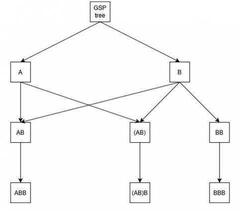
For example, the ‘AA’ item is found in two sequence transactions SID #1 (<A,B,(AB),B,C>), and #2(<(AB), B, B,(AC), C>), while absent in SID #3 (<(AB), B, B, B, B>). The fifth step is to create all the possible three-item candidate nodes. The passed support criteria for two-item nodes will be used to generate the three-item candidate node. For example, the two items that passed the support criteria ‘AB’ will be separated into the first and second items as ‘A’ and ‘B’. After passing the support criteria node, the last item, ‘B’, will be considered to combine with the previous two items. From Table 6, for example, one node of the two items passed the support criteria, ‘AB’. Thus, the last item ‘B’ will combine with ‘BB’ to form the new two-item candidate node. The 2-item ‘BB’ is chosen to be put in the back of ‘B’ since it passed the support criteria, Table 6. Then, this new two-item candidate node will be preceded by the first letter ‘A’ to create the candidate three-item node, ‘ABB’. Each candidate's item node must be checked for validity (pruning). For example, ‘ABB’ is decomposed to ‘AB’, ‘BB’, and ‘AB’. These parts are measured to determine whether the support value is equal. In this case, the support values of ‘AB’=3, ‘BB’=3, and ‘AB’=3, thus all parts have equal support numbers. Therefore, this three-item candidate passed the validity test. If the validity check reveals that they are not equal, then this candidate will be pruned or purged. After that, the three-item candidate node will be checked against all the sequence transactions of all SIDs to determine whether the three-item candidate nodes can pass the support criteria, as shown in Table 8.
Table 8. The possible two-item node with a support number result
|
-3-Item Node |
Last |
2 Item (Support Passed) |
First |
Composed |
Prune Checking |
Support |
Pass-p |
|
AB |
B |
BB |
A |
ABB |
p |
3 |
p |
|
BB |
B |
BB |
B |
BBB |
p |
3 |
p |
|
(AB) |
B |
BB |
A |
(AB)B |
p |
3 |
p |
|
|
A |
AB |
B |
(AB)B |
|
|
|
Table 9. The possible four items node with a support number result
|
-4-Item |
Last |
3 Item (Support Passed) |
First |
Composed |
Validity Checking |
Support |
Pass-p |
|
ABB |
BB |
BBB |
A |
ABBB |
p |
2 |
f |
|
BBB |
BB |
BBB |
B |
BBBB |
p |
1 |
f |
|
(AB)B |
AB |
ABB |
B |
BABB |
- |
||
|
BB |
BBB |
A |
ABBB |
The sixth step is to create all the possible four-item candidate nodes. Since three items support the passed criteria, ‘ABB’, ‘BBB’, and ‘(AB) B’, the fourth candidate node must be further defined. The solution for the four-item generating is to follow the same steps as step five. The difference between this step and step five is that the source three-item node must be separated from the last two items to be used as the predecessor of the three-item node generation. Then, these three generated nodes will be preceded by the first letter. The validity of each part of the four-item candidate node is checked. The pass validity checking four-item candidate node will be checked for its support number if it meets the support criteria. The result of the sixth step calculation is presented in Table 9. No four-item candidate node passes the support criteria, even though two of them pass the validity check, “ABBB” and “BBBB”. Therefore, there is no need to generate the five-item candidate node since no four-item nodes meet the support criteria.
In summary, Figure 1 illustrates an n-item node relationship structure that passed the support criteria tree.
Figure 1. The n-item node relationship tree of GSP analysis (support number criteria ≥3)
2.4 Markov chains and a research practical example
A) Markov chains concept
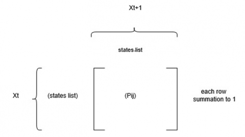
If Xt is the process as shown in Figure 2, for example, several states ‘i’ at time ‘t’.The process of state ‘i’ at time t, Xt, is presented as Xt=i. The process space {X0, X1,….Xn} represents the process Xt that varies from time t=0 to n, where ‘n’ is the size of the process space. If process Xt depends on only process Xt-1, but not on the past Xt-2,…Xt0, then these processes are called Markov Chains [10]. The transition state [11] space from time ‘t’ to time ‘t+1’, which processes xt to xt+1, is presented with its probability in the transition matrix. P=(pij), i and j =1,…, n is the transition matrix from each state at process Xt to all the states in Xt+1. The total probability of each state at row i to every state in columns 1, 2, … n has a total value of 1.0.
Figure 2. Markov chain concept
B) Markov chain - practical example
From the transaction of all sequence IDs in Table 7 and the sequence of items that occurred, Figure 1 is used to obtain the frequency of the item relationship. All the frequencies of item relationships are presented in Table 10.
Table 10. The frequency of item relationships from a particular row to all items in all columns
|
A |
B |
AB |
BB |
(AB) |
ABB |
BBB |
(AB)B |
|
|
A |
0 |
4 |
0 |
3 |
0 |
0 |
2 |
0 |
|
B |
2 |
8 |
1 |
3 |
1 |
0 |
2 |
1 |
|
AB |
1 |
3 |
1 |
2 |
1 |
0 |
1 |
1 |
|
BB |
1 |
5 |
0 |
2 |
0 |
0 |
1 |
0 |
|
(AB) |
0 |
3 |
0 |
2 |
0 |
0 |
1 |
0 |
|
ABB |
1 |
2 |
0 |
1 |
0 |
0 |
0 |
0 |
|
BBB |
1 |
2 |
0 |
1 |
0 |
0 |
0 |
0 |
|
(AB)B |
0 |
2 |
0 |
1 |
0 |
0 |
1 |
0 |
For example, frequency counting from item ‘A’ to ‘A’ can be obtained from the number of occurrences that start with ‘A’, then suddenly followed by item ‘A’. Since this situation did not occur, frequency A-A, thus fA-A, is zero. In the following example, the frequency counting from item ‘BB’ to ‘B’ can be obtained from the number of occurrences that start with ‘B’, then suddenly followed by item ‘BB’. The result of counting is five given source and destination item patterns matching. A detailed explanation of the counting of matching item relationships is presented in Table 11.
Table 11. Example of item results counting
|
SID |
Item-Sequence-Source |
Couple of Item-Result |
|
1 |
<A,B,(AB),B,C> |
$<A, \bar{B},(A \bar{B}), \underline{B}, C>$ |
|
2 |
<(AB),B,B,(AC),C> |
$<(A \bar{B}), \bar{B}, \underline{B},(A C), C>$ |
|
3 |
<(AB),B,B,B,B> |
$<(A \bar{B}), \bar{B}, \underline{B}, B, B>$ |
|
3 |
|
$<(A B), \bar{B}, \bar{B}, \underline{B}, B>$ |
|
3 |
|
$<(A B), B, \bar{B}, \bar{B}, \underline{B}>$ |
2.5 Likelihood of a hidden Markov chain on damage occurring notification (alert)
The frequency of item relationships from a particular row to all items in all columns in Table 10 is transformed into a transition matrix as illustrated in Table 12.
Table 12. Transition matrix of sample data
|
|
A |
B |
AB |
BB |
(AB) |
ABB |
BBB |
(AB)B |
|
A |
0.000 |
0.444 |
0.000 |
0.333 |
0.000 |
0.000 |
0.222 |
0.000 |
|
B |
0.111 |
0.444 |
0.056 |
0.167 |
0.056 |
0.000 |
0.111 |
0.056 |
|
AB |
0.100 |
0.300 |
0.100 |
0.200 |
0.100 |
0.000 |
0.100 |
0.100 |
|
BB |
0.111 |
0.556 |
0.000 |
0.222 |
0.000 |
0.000 |
0.111 |
0.000 |
|
(AB) |
0.000 |
0.500 |
0.000 |
0.333 |
0.000 |
0.000 |
0.167 |
0.000 |
|
ABB |
0.250 |
0.500 |
0.000 |
0.250 |
0.000 |
0.000 |
0.000 |
0.000 |
|
BBB |
0.250 |
0.500 |
0.000 |
0.250 |
0.000 |
0.000 |
0.000 |
0.000 |
|
(AB)B |
0.000 |
0.500 |
0.000 |
0.250 |
0.000 |
0.000 |
0.250 |
0.000 |
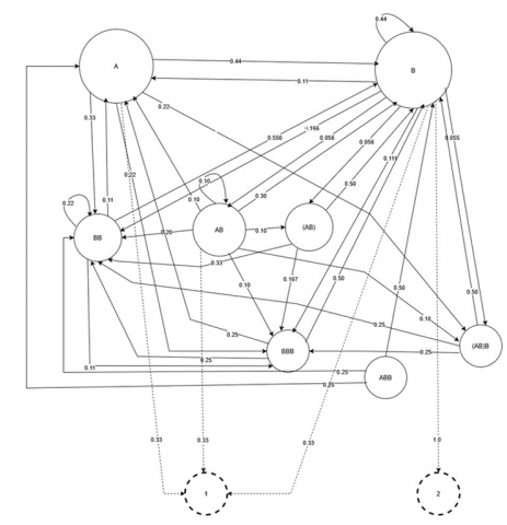
The transition matrix in the Markov chain is shown in Figure 3. The State or item sequence transaction in Table 7 showed the items or states of each user, which were categorized by day. During the phase of learning about security risks, the DB administrator (DBA) must monitor whether any undesirable incidents are occurring. On the day any incident occurs, DBA will collect all the transaction records for that date. This evidence defines its type of risk. The findings will be recorded to gain knowledge of security risk. The likelihood of the risk is determined based on the undesirable incident's effective items. For example, if there are two undesirable incidents occurred in date # 1, #2 and #3 with risk types ‘1’, and ‘2’, thus the significant item and likelihood which related to the incident ‘1’, ‘2’, and ‘1’ are (‘A’=0.33, ‘B’=0.33, ‘(AB)’=0.33), (‘B’=1.0), and(‘A’=0.33, ‘B’=0.33, ‘(AB)’=0.33), in respectively, as shown in Table 13, and Figure 3.
Table 13. The related item that occurred on the same date as the security incident
|
Date |
1 |
2 |
3 |
4 |
|
List |
A (0.33) |
B(1.0) |
(AB) |
C |
|
of |
B (0.33) |
B |
A |
C |
|
items |
(AB)(0.33) |
B |
B |
B |
|
Risk type |
-1- |
-2- |
-1- |
No |
Figure 3. Hidden Markov chain of sample data
Only item ‘B’, which is simultaneously used by three users, causes the probability of risk occurring to be ‘2’.
The stable state vector is calculated from its transition matrix. This vector will provide information about the stability or steady likelihood. This vector provides the amount of each state at the stable state probability if the total state or item is known. Assume that there are 100 items in the scope of the calculation; Therefore, the amount of each state at the stable state is shown in Table 14.
Table 14. The amount of each item is based on the steady probability and the total amount. of state (e.g., ‘n’=100)
|
State |
State-A |
State-B |
5 |
State-BB |
State-(AB) |
State-ABB |
State-BBB |
State-(AB)B |
|
Steady probability (S) |
0.108 (SA) |
0.473 (SB) |
0.029 (SAB) |
0.214 (SBB) |
0.029 (S(AB)) |
0 (SABB) |
0.115 (SBBB) |
0.0295 (S(AB)B)) |
|
Amount of item occurring (n) |
10.82 |
47.36 |
2.95 |
21.46 |
2.95 |
0 |
11.53 |
2.95 |
If DBA has defined that the red line of undesirable incident will do alert at eighty percent of the number of items occurring (N), therefore: Rule-1, and Rule-2 for risk type 1, 2 prevention are: Rule-1: If [number of item ‘A’ > (0.80*NA*SPA) .and. number of ‘B’> (0.80*NB*SPB). and. number of ‘(AB)’>0.80*NAB*SPAB)] then print “***Alert-Risk-1***”. Rule-2: If [amount of item ‘B’ > (0.80*NB*SPB)] then print “***Alert-Risk-2***”. Where, for example, NA is the number of item ‘A’ under the stable probability of item ‘A’, SPA.
2.6 Related research
A) ISO-27001
ISO-27001 [12] is a popular widely recognize standard that provides the framework for an information security management system. These standards are applied to enhance the security of the organization’s database. The ISO-27001 standard features cover security risk management, access control, data integrity, monitoring and logging, security awareness and training, etc.
B) Efficient storage and querying of sequential patterns in database systems
The sequential patterns generated from an original database become a massive collection of sequential patterns [13]. Many pattern discovery tools, such as DB-Miner, can generate an enormous amount of information. The various views of these patterns provide necessary details for capturing insights. The methods of storing these whole sequential patterns are proposed by effective pattern coding.
C) Trust factor-based analysis of user behavior using sequential pattern mining for detecting intrusive transactions in databases
Malicious access and modifications to databases by insider employees [14] are tough to detect and prevent. Some have attempted to escalate their privileges, while many have exploited SQL commands for database attacks. The pattern of the insider threat can be derived from the SQL commands used and database log examinations. The research results present the trust factor of the SQL command used by the user. Some users who deviate from the trust factor will be assumed to be an insider threat.
D) Database security and encryption
A Survey Study [15]. The user’s authorization always controls the integrity of database manipulation. Some intruders try to escalate their approval or secretly use another user's trustee rights. A simple solution to this problem is to add user authentication verification and database encryption. This method can discriminate between those who cause the database fault or failure.
E) Database security threats and how to mitigate them
A database security breach [16] can involve malicious access by an insider or an outsider organization. A database administrator takes responsibility for the database. He must have experience with database command vulnerabilities or dangers so that the failures or faults can be detected and corrected, ROLLBACK. Nevertheless, security attacks come from many sources. The manager must be concerned about the database security policy and tightly govern it to reduce and control vulnerabilities.
F) Advancing database security: A comprehensive systematic mapping
In total, 20 challenges related to database security [17] were identified. Research results show that ‘‘weak authorization system, ‘‘weak access control, ‘‘privacy issues/data leakage, ‘‘lack of NOP security, and ‘‘database attacks’’ are the most frequently cited critical challenges. Further analyses were performed to highlight the different difficulties associated with various phases of the software development lifecycle, venues of publications, types of database attacks, and active research institutes/universities researching database security. Organizations should implement adequate mitigation strategies to address the identified database challenges.
G) Sequential pattern analysis for event-based intrusion detection
Many events utilize computer resources, including databases, peripherals, and networks. Some events are intended to access the organization's database maliciously, etc. [18]. The behavior of user events (commands used) creates their processing patterns. The pattern with class attributes is composed to create a cluster of normal behavior users and distinguish them from unnatural users. The generalized sequential pattern (GSP) is used to seek SQL behavior patterns.
H) Database intrusion detection using role and user level sequential pattern mining and fuzzy clustering
The behavior of each database user [19] is examined to determine whether they are working correctly under the assigned rights. If he tries to work contrary to the assigned authority, this user will be flagged for careful observation. The use of SQL commands could cause an undesirable incident. Thus, the sequential pattern of his work with the data processing result examined will support the criteria for whether the user intends to access the data maliciously.
I) SQL injection hacking
SQL injection is a type of database intrusion that compromises sensitive information assets. There are some kinds of dangerous SQL commands [20]. These commands will be sent or injected to execute in the DBMS to retrieve some desirable information. The vulnerability of the DBMS will be detected before the intruder considers the capable SQL command to attack the DBMS.
J) Maintainability measurement
The system broke down due to an interruption in business operations. The clash system has to be repaired and restored to the normal state. The DBAs have to be concerned about at least two indexes. The first item is Mean time between failure, also known as MTBF [21]. The MTBF is used to measure the average time between system failures during a period. If MTBF is a small number of time (Tmtbf), then further failures shall occur on about T unit of time from the current time, e.g., T0, as To+Tmtbf. The MTBF can be obtained from the formula: MTBF=Total operation time/ number of system breakdowns. The second item is Mean time to repair, aka MTTR [22]. The MMTR is used to measure the average repair time. With the large number of MTTR, the system will resume normal working, which will take a long time to repair, Tmttr. The formula to obtain the MTTR: MTTR(Tmttr)=Total number of downtimes/total number of system breakdowns. The DBAs must be concerned about the root cause of failures, problem-solving, gaining the best practice solution to prevent, and proactively preventing these possible causes of failures.
3.1 Research context (experimental sample, DB sample, MySQL, duration of data collection)
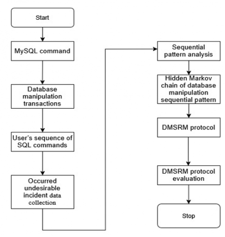
The overall activity of this research is shown in Figure 4.
Figure 4. Research flowchart
The experimental sample is the computer department of a private agricultural product domestic merchandising company in Thailand. The research was conducted in December 2024. Three organizational IT-DB users are responsible for database manipulation. The overall digital and database knowledge, skills, and intelligence are low to medium. Therefore, these users might not carry out the intended activity in a database security attack. However, on some occasions, the combination of multiple SQL commands working simultaneously may cause failure or even compromise the DB management system. This organization uses MySQL as a database server. Therefore, the result of this study may differ from that of another organizational database management system. Hence, it is not suitable to reference this research result directly in another. The proposed solution presents a step-by-step calculation that can be applied to those who need to solve a similar problem.
The research limitation was studied in one department. To increase the reliability of the proposed solution, it was developed in late November 2024 and will be used on-site for three months (December 2024, January 2025, February 2025, and March 2025). The data results of DMSRD for each month were gathered. DBAs analyzed the errors or problems encountered during the first month to identify the causes of failures, thereby preventing this pattern of dangerous SQL commands and utilizing this knowledge to create alert rule settings. At the end of the second month of DMSRD use, the sequential pattern, Hidden Markov chain, and alert rule were recalculated. The second newly generated rule will be used to monitor undesirable people in the third month. The repetitive recalculation will be finished if the solution maintainability index measuring (e.g., MTBF, MTTR) meets the organization’s preference criteria. The experiment is summarized in topic 4.6.
3.2 Working table (user’s SQL used statements, transaction, undesirable incident, HMM)
Many SQL commands contain various options and features. SQL command defects can occur when using some SQL commands in a specific command form, which could cause a violation or a critical loss of sensitive data. Some users have less experience writing SQL commands, which could lead to undesirable security incidents on the DBMS. The patterns of SQL command writing that could cause the problems should be systematically recorded to use them for security risk monitoring, awareness, and prevention. This research will primarily focus on using SQL commands without considering the associated risks. The SQL commands in this research include the fundamental SQL commands: CREATE, INSERT, SELECT, UPDATE, DELETE, and GRANT.
3.3 Steps of research
The details of the research steps are explained below.
3.3.1 Scope of MySQL commands
The SQL command research has limited coverage, and its Symbols are presented in Table 15.
Table 15. Research is limited on SQL commands
|
Symbol |
Detail |
|
A |
CREATE table |
|
B |
INSERT |
|
C |
SELECT |
|
D |
UPDATE |
|
E |
DELETE record |
|
F |
GRANT |
|
Minimum SUPPORT number |
3 |
3.3.2 User’s sequence of database manipulation transactions
The SQL commands for all three DB users' experiments were retrieved from the DB manipulation logs table. These data are rearranged according to the transaction date of SQL commands used by each DB user, as shown in Table 16. The data were collected on six working days per week and twelve hours per day in the fourth week of the month. In the last week of each month, many vital data processing transactions are always busy, which must be completed and processed before the end of the month.
Table 16. SQL command used a sequence of three organizational DB users in eight days of the week for the fourth week of the month
|
Transaction Date |
User-ID |
SQL-Command Used |
SQL-Command used Sequence |
|
1 |
1 |
A,F |
<(AF),B,B,C,(CD),D,E,C> |
|
2 |
1 |
B |
|
|
3 |
1 |
B |
|
|
4 |
1 |
C |
|
|
5 |
1 |
CD |
|
|
6 |
1 |
D |
|
|
7 |
1 |
E |
|
|
8 |
1 |
C |
|
|
1 |
2 |
A |
<A,B,E,C,(CD),C,(DF),B> |
|
2 |
2 |
B |
|
|
3 |
2 |
E |
|
|
4 |
2 |
C |
|
|
5 |
2 |
CD |
|
|
6 |
2 |
C |
|
|
7 |
2 |
DF |
|
|
8 |
2 |
B |
|
|
1 |
3 |
A |
<A,B,B,B,(DF),E,(CD),C> |
|
2 |
3 |
B |
|
|
3 |
3 |
B |
|
|
4 |
3 |
B |
|
|
5 |
3 |
DF |
|
|
6 |
3 |
E |
|
|
7 |
3 |
CD |
|
|
8 |
3 |
C |
|
3.3.3 User’s sequence of database manipulation sequential pattern analysis
The SQL command sequence experimental data was used to extract the sequential pattern using the GSP algorithm. The one-item sequential pattern is presented in Table 17. Six items passed the support criteria (‘3’).
Table 17. One item SQL used a command sequential pattern
|
- 1 Item- |
Description |
Support |
Pass-p |
|
A |
CREATE table |
3 |
p |
|
B |
INSERT |
3 |
p |
|
C |
SELECT |
3 |
p |
|
D |
UPDATE |
3 |
p |
|
E |
DELETE record |
3 |
p |
|
F |
GRANT |
3 |
p |
The six passed support numbers were discovered to have a two-item sequential pattern. Fourteen two-item patterns have the support number equal to ‘3’, as shown in Table 18.
Table 18. Two items SQL used command sequential patterns
|
-2 Item- |
Support |
Pass |
|
AB |
3 |
p |
|
AC |
3 |
p |
|
AD |
3 |
p |
|
AE |
3 |
p |
|
BB |
3 |
p |
|
BC |
3 |
p |
|
BD |
3 |
p |
|
BE |
3 |
p |
|
CC |
3 |
p |
|
CD |
3 |
p |
|
DC |
3 |
p |
|
DD |
3 |
p |
|
EC |
3 |
p |
|
(CD) |
3 |
p |
Table 19. Three items SQL used the command sequential patterns
|
-3- Item |
2-seq-1st |
2-seq (2) |
2-seq-Last |
3-seq After Join |
3-seq After Prune (Pass) Fail-Blank |
Support |
Pass |
|
AB |
B |
BB |
A |
ABB |
ABB |
3 |
p |
|
|
|
BC |
|
ABC |
ABC |
3 |
p |
|
|
|
BD |
|
ABD |
ABD |
3 |
p |
|
|
|
BE |
|
ABE |
ABE |
3 |
p |
|
AC |
C |
CC |
A |
ACC |
ACC |
3 |
p |
|
|
|
CD |
ACD |
ACD |
2 |
|
|
|
AD |
D |
DC |
A |
ADC |
ADC |
2 |
|
|
|
|
DD |
|
ADD |
ADD |
3 |
p |
|
AE |
E |
EC |
A |
AEC |
AEC |
3 |
p |
|
BB |
B |
BB |
B |
BBB |
BBB |
1 |
|
|
|
|
BC |
|
BBC |
BBC |
2 |
|
|
|
|
BD |
|
BBD |
BBD |
2 |
|
|
|
|
BE |
|
BBE |
BBE |
2 |
|
|
BC |
C |
CC |
B |
BCC |
BCC |
3 |
p |
|
|
|
CD |
|
BCD |
BCD |
2 |
|
|
BD |
D |
DC |
B |
BDC |
BDC |
3 |
p |
|
|
|
DD |
|
BDD |
BDD |
3 |
p |
|
BE |
E |
EC |
B |
BEC |
BEC |
3 |
p |
|
CC |
C |
CC |
C |
CCC |
CCC |
2 |
|
|
CD |
D |
|
C |
CCC |
|
|
|
|
DC |
C |
CC |
D |
DCC |
DCC |
1 |
|
|
|
|
CD |
|
CDD |
2 |
|
|
|
|
|
|
|
||||
|
DD |
D |
DC |
D |
DDC |
DDC |
1 |
|
|
|
|
DD |
|
DDD |
DDD |
0 |
|
|
EC |
C |
CC |
E |
ECC |
ECC |
2 |
|
|
(CD) |
D |
DC |
C |
(CD)D |
2 |
|
|
|
|
|
DD |
|
(CD)D |
|
||
|
|
C |
CC |
D |
(CD)C |
(CD)C |
3 |
p |
|
|
|
D |
(CD)C |
|
|||
|
|
|
CD |
|
(CD)D |
|
The fourteen two-item patterns were further examined for their three-item sequential patterns; twelve three-item patterns could pass the prune checking (or validity), counting, and ≥ support number criteria, as shown in Table 19.
These twelve three-item sequential patterns were further discovered for their four-item sequential patterns. Two three-item sequential patterns can pass the prune checking, and the support number is ≥3. The four candidate items SQL used command sequential patterns are presented in Table 20.
Table 20. Four items SQL used command sequential patterns
|
-4 Item |
3-seq-1st |
3-seq (2) |
3-seq-Last |
4-seq After Join |
4-seq After Prune (Pass) |
Support |
Pass |
|
ABD |
BD |
BDC |
A |
ABDC |
ABDC |
3 |
p |
|
|
|
BDD |
|
ABDD |
ABDD |
3 |
p |
Table 21. Five items SQL used command sequential patterns
|
-5- (1) |
4-seq-1st |
4-seq (2) |
4-seq-Last |
5-seq After Join |
5-seq After Prune |
Support |
Pass |
|
ABCC |
BCC |
- |
A |
|
|
||
|
ABDC |
BDC |
- |
A |
|
|
|
|
|
ABDD |
BDD |
- |
A |
|
|
|
The two four-item sequential patterns were continued to be derived for the five-item sequential pattern; however, no five-item sequential patterns could pass the support criteria, as shown in Table 21.
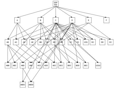
3.3.4 GSP tree of n-items sequential patterns
The results of the derived n-item sequential patterns relation were illustrated in Figure 5. Figure 5 shows that one-item nodes ‘B’, ‘C’, and ’D’ were the essential nodes frequently used. ‘AB’ is the two-item node that was the prior node of many other three-item nodes.
The summary of the n-item sequential pattern (Figure 5) and the SQL command used to sequence three organizational DB users (Table 16) were used to obtain the transition probability, as shown in Table 22. The stable states vector of the sample research matrix is shown in Table 23.
Figure 5. GSP of the research sample case study
Table 22. Transition matrix of sample research
|
A |
B |
C |
D |
E |
F |
AB |
BB |
BC |
CD |
DC |
DF |
EC |
(CD) |
ABB |
ABE |
BCC |
BEC |
BCC |
(CD)C |
|
|
A |
0 |
1 |
0 |
0 |
0 |
0 |
0 |
0 |
0 |
0 |
0 |
0 |
0 |
0 |
0 |
0 |
0 |
0 |
0 |
0 |
|
B |
0 |
0.375 |
0.125 |
0.125 |
0.125 |
0.125 |
0 |
0 |
0 |
0 |
0 |
0.125 |
0 |
0 |
0 |
0 |
0 |
0 |
0 |
0 |
|
C |
0 |
0.308 |
0.3077 |
0 |
0.077 |
0 |
0 |
0 |
0.077 |
0 |
0.076 |
0 |
0.153 |
0 |
0 |
0 |
0 |
0 |
0 |
|
|
D |
0 |
0.143 |
0.286 |
0.142 |
0.285 |
0 |
0 |
0 |
0 |
0.143 |
0 |
0 |
0 |
0 |
0 |
0 |
0 |
0 |
0 |
0 |
|
E |
0 |
0 |
0.429 |
0.142 |
0 |
0 |
0 |
0 |
0 |
0.143 |
0.143 |
0 |
0 |
0.142 |
0 |
0 |
0 |
0 |
0 |
0 |
|
F |
0 |
0.667 |
0 |
0 |
0.333 |
0 |
0 |
0 |
0 |
0 |
0 |
0 |
0 |
0 |
0 |
0 |
0 |
0 |
0 |
0 |
|
AB |
0 |
0.667 |
0 |
0 |
0.333 |
0 |
0 |
0 |
0 |
0 |
0 |
0 |
0 |
0 |
0 |
0 |
0 |
0 |
0 |
0 |
|
BB |
0 |
0.2 |
0.2 |
0.2 |
0 |
0.2 |
0 |
0 |
0 |
0 |
0 |
0.2 |
0 |
0 |
0 |
0 |
0 |
0 |
0 |
0 |
|
BC |
0 |
0 |
0.333 |
0.333 |
0 |
0 |
0 |
0 |
0 |
0.333 |
0 |
0 |
0 |
0 |
0 |
0 |
0 |
0 |
0 |
0 |
|
CD |
0 |
0.333 |
0.333 |
0.333 |
0 |
0 |
0 |
0 |
0 |
0 |
0 |
0 |
0 |
0 |
0 |
0 |
0 |
0 |
0 |
0 |
|
DC |
0 |
0 |
0 |
0 |
0 |
0 |
0 |
0 |
0 |
0 |
1 |
0 |
0 |
0 |
0 |
0 |
0 |
0 |
0 |
0 |
|
DF |
0 |
0 |
0 |
0 |
0 |
0 |
0 |
0 |
0 |
0 |
0 |
1 |
0 |
0 |
0 |
0 |
0 |
0 |
0 |
0 |
|
EC |
0 |
0 |
0.5 |
0.25 |
0 |
0 |
0 |
0 |
0 |
0.25 |
0 |
0 |
0 |
0 |
0 |
0 |
0 |
0 |
0 |
0 |
|
(CD) |
0 |
0 |
0.667 |
0.333 |
0 |
0 |
0 |
0 |
0 |
0 |
0 |
0 |
0 |
0 |
0 |
0 |
0 |
0 |
0 |
0 |
|
ABB |
0 |
0.5 |
0.5 |
0 |
0 |
0 |
0 |
0 |
0 |
0 |
0 |
0 |
0 |
0 |
0 |
0 |
0 |
0 |
0 |
0 |
|
ABE |
0 |
0 |
1 |
0 |
0 |
0 |
0 |
0 |
0 |
0 |
0 |
0 |
0 |
0 |
0 |
0 |
0 |
0 |
0 |
0 |
|
BCC |
0 |
0 |
0 |
1 |
0 |
0 |
0 |
0 |
0 |
0 |
0 |
0 |
0 |
0 |
0 |
0 |
0 |
0 |
0 |
0 |
|
BEC |
0 |
0 |
1 |
0 |
0 |
0 |
0 |
0 |
0 |
0 |
0 |
0 |
0 |
0 |
0 |
0 |
0 |
0 |
0 |
0 |
|
BCC |
0 |
0 |
0 |
1 |
0 |
0 |
0 |
0 |
0 |
0 |
0 |
0 |
0 |
0 |
0 |
0 |
0 |
0 |
0 |
0 |
|
(CD)C |
0 |
0 |
0 |
0 |
0 |
0 |
0 |
0 |
0 |
0 |
0 |
1 |
0 |
0 |
0 |
0 |
0 |
0 |
0 |
0 |
Table 23. Stable state vector of sample research
|
7 |
B |
C |
D |
E |
F |
AB |
BB |
BC |
CD |
DC |
DF |
EC |
(CD) |
ABB |
ABE |
BCC |
BEC |
BCC |
(CD)C |
|
0 |
0.241 |
0.174 |
0.121 |
0.124 |
0.056 |
0. |
0 |
0 |
0.045 |
0.018 |
0.1814 |
0 |
0.037 |
0 |
0 |
0 |
0 |
0 |
0 |
4.1 User’s sequence of database manipulation, sequential pattern analysis
1) Transition matrix
The summary of the n-item sequential pattern (Figure 5) and the SQL command used to sequence three organizational DB users (Table 13) were used to obtain the transition probability. The transition matrix of the n-item sequential pattern of the sample research pattern is presented in Table 19.
2) Stable transition vector
The transition matrix was calculated for the steady or stable state vector, as shown in Table 20. The stable transition vector will obtain the number of items that occur when the total number of used items is given from actual item counting or prediction.
4.2 Occurred undesirable incident data collection and Markov chain of database manipulation sequential pattern
A DB administrator takes responsibility for database performance and security preservation. In the event of an undesirable security incident, he must retrieve all the SQL commands that were used when the security loss occurred. For example, two undesirable security incidents occurred on day ‘5’, and ‘7’. From Table 24, date # ‘5’, Risk ‘1’ occurred while node ‘2*(CD)’ and ‘1*(DF)’ worked on day # ‘5’. Thus the probability of ‘(CD)’ was 0.66, while ‘(DF)’ was 0.33. On date #7, the Risk ‘2’ happened when n-items ‘E’, ‘DF’, and ‘CD’ were used simultaneously. Thus, the probability of ‘E’ was 0.33, ‘(DF)’ was 0.33, and ‘(CD)’ was 0.33.
Table 24. An undesirable security incident occurred in the sample research
|
|
Day of Week 1-8 |
|||||||
|
User ID |
1 |
2 |
3 |
4 |
5 |
6 |
7 |
8 |
|
1 |
(AF) |
B |
B |
C |
(CD) (0.33) |
D |
E(0.33) |
C |
|
2 |
A |
B |
E |
C |
(CD)(0.33) |
C |
(DF)(0.33) |
B |
|
3 |
A |
B |
B |
B |
(DF)(0.33) |
E |
(CD)(0.33) |
C |
|
Occurred damage incident |
- |
- |
- |
- |
1 |
- |
2 |
- |
1) Undesirable security incident
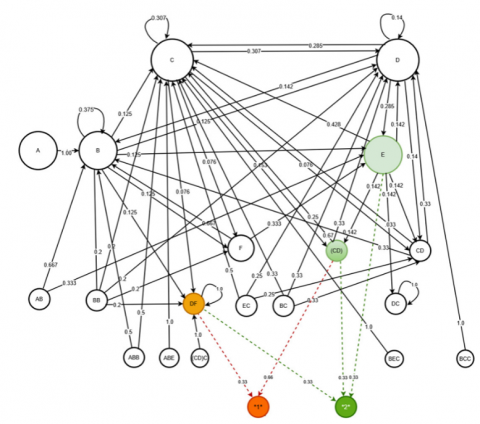
2) Hidden Markov chain of undesirable security incidents occurring in the sample research
The plain Markov chain was enhanced with the actuator nodes ‘1’ alert and ‘2’ alert. The hidden Markov chain was presented in Figure 6.
Figure 6. Hidden Markov chain of sample research
Note that some item nodes from the n-item sequential pattern in the GSP tree disappear in the hidden Markov chain because no events match the Markov chain rule of state (2.4), e.g., ‘ABDC’ and ‘ABDD’.
3) Rule of undesirable security incident occurring alert
The result of the Hidden Markov chain and stable transition matrix can be derived the rule as shown in pseudo code (1), and (2).
(1) Rule-1:
IF [number of item ‘DF’ >(0.80*NDF*0.33) and the number of item ‘CD’ > (0.80*NCD*0.66), then print “Alert undesirable security incident *1*”.
(2) Rule-2:
IF [number of item ‘DF’ > (0.80*NDF*0.33) and the number of item ‘CD’ > (0.80*NCD*0.33) and number of item ‘E’ > (0.80*NE*.33), then print “Alert undesirable security incident *2*”.
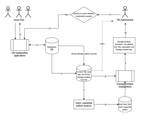
4.3 Database manipulation security risk detection protocol (DMSRD)
The scenario of the DMSRD protocol's tasks is illustrated in Figure 7. Two additional tables keep the necessary data for sequential pattern analysis and rule-based alert detection. Tables 25 and 26 detail the two extra tables for DMSRD support. Table A: This additional file will continuously receive (step #3) the details of the SQL command used by the DB user on the organizational DB (steps #1 and #2). The DBMS’s condition of data manipulation states are retrieved by the procedure ‘Damage incident management’. These states will be in the column ‘State of DB processing’ in the ‘table A’- the state of DB processing. If any undesirable incident occurs, the code will be set to ‘2’, while ‘1’ represents a normal situation.
Figure 7. DMSRD protocol
Table 25. Details of table A. User’s SQL used logs, and (if any) damage incidents occurred
|
|
Time-Stamp |
User -ID |
SQL Command |
Detail of SQL Command |
State of DB Processing |
|
Data type |
Y-M-D |
Department (A, B, C) (A=accounting, B=Sales, C= Stock control) |
SQL Data manipulation, Data definition, Data control, and Data query definition: (CREATE, INSERT, UPDATE, DELETE, and SELECT)I |
Detail of full SQL statement |
1: Normal 2: If there are any undesirable incident occurred |
|
E.g. |
2025-01-9 |
A:01 |
CREATE TABLE |
CREATE TABLE Employee (EmployeeIdint NOT NULL, FirstNamevarchar(20) NOT NULL, LastNamevarchar(20) NOT NULL, PhoneNumbernvarchar(10) NULL, PositionIdint NOT NULL) |
1 |
Table 26. Detail of table B. All users’ SQL used a sequential pattern
|
|
Start Time-Stamp |
Stop Time-Stamp |
Sequential Node-1 |
Sequential Node-2 |
Supports |
|
Description |
Y-M-W-D |
Y-M-W-D |
The first node |
The second node |
The number of possible matched sequence of node |
|
E.g. 1 |
2025-01-1-9 |
2025-01-1-16 |
A |
A |
0 |
|
… |
2025-01-1-9 |
2025-01-1-16 |
A |
B |
3 |
|
… |
2025-01-1-9 |
2025-01-1-16 |
A |
E |
3 |
|
… |
..... |
..... |
..... |
..... |
..... |
|
… |
2025-01-1-9 |
2025-01-1-16 |
A |
BDD |
3 |
The data on SQL commands used, from table B, were calculated for all n-item sequential patterns (step #5). The cumulated SID will be used to derive the current sequential pattern of n items (step #6), all of which will be kept in table B. The sequential pattern of n-items will be read from the ‘Damage incident management procedure’ (step #7). The transition probability matrix, stable transition probability vector, and Markov chain were generated. ‘Damage incident management’ procedure read table ‘A’, as shown in Table 26.
DMSRD protocol brief explanation: (two actors, DB users, and DBA)
1: DB users manipulate their authorized data in the organizational database through the application or a direct connection.
2: The DB users’ commands are sent to process their request in the DB. If the trustee rights checking is passed, the requesting command is permitted to run on the organizational DB.
3: The used SQL command and its details are kept in table A.
4: If there is any damage or undesirable security incident, the risk type number of the arising risk will be appended to the column ‘State of DB processing’, for example, ‘1’.
5: The User sequence item transactions (SID) are used to discover the n-item sequential pattern analysis.
6: The discovered n-item sequential patterns are kept in table B.
7: The discovered n-item sequential patterns are sent to ‘Damage incident management’ under the specified time duration. This procedure will derive the Markov chain and stable transition probability vector.
8: The undesirable security incident risk type number (if there are any) is mapped to all users’ n-item sequence transactions. The probability of the effective nodes is calculated. The stable transition matrix (7) and ‘N’ or total number of used items are used to derive the Hidden Markov chain and risk security alert rules.
9: The DBA will use the defined rules of the security incident alerts to detect potential security incidents.
10: The defined rules of security incident alerts are sent to the DBA.
11: If some not-appreciated evident possibilities could happen (10* notification), the DBA will configure some activity to the DB manipulation application, such as delaying or purging some user’s command from the ready queue, etc.
12: The configuration from the DBA will be managed by the DBA under the DBA’s role-based control.
13: The reaction message about the inconvenience of the user’s DB manipulation is sent to the current DB application and to particular DB users.
4.4 Protocol evaluation
The DMSRD protocol was validated for its accuracy in mitigating undesirable security risk incidents on eight additional days, while also demonstrating effectiveness over one-week period. Table 27 presents DBA’s define the risk type.
Table 27. The code of the risk type
|
Risk Type |
Alert Code |
|
Privilege Escalation |
1 |
|
Inject false records or manipulate data lineage, data inconsistencies. |
2 |
|
Modify sensitive data (Integrity loss), Data tampering |
3 |
|
Data loss, sabotage, removal of all the table's records |
4 |
|
Mass data extraction |
5 |
|
Unable to identify |
9 |
The detection accuracy of risk type (‘1, 2, 3, 4, 5, 9’) was approximately 73.68%, as shown in Table 28.
Table 28. Accuracy of undesirable security incident detection
|
Test-record# |
Risk Type |
Correct Alert |
In Correct Alert |
|
14 |
1 |
12 |
2 |
|
12 |
2 |
8 |
4 |
|
16 |
3 |
13 |
3 |
|
20 |
4 |
12 |
8 |
|
14 |
5 |
11 |
3 |
|
Total |
|
56 |
20 |
|
Percent |
|
73.68 |
26.32 |
4.5 MTBF and MTTF
The DMSRD proposed protocol is for deployment in the organization for real database manipulation. The experiment was conducted over a four-month period. In the first month of DMSRD use, no defined sequential patterns, a Hidden Markov chain, and a rule for security risk alert. This month's number#1 was the duration of the item sequence, undesirable incident gathering. At the end of the first month of DMSRD use, the rule for an undesirable security incident alert will be created. This month, MTBF and MTTR were the worst numbers. DBAs will consider the combination of SQL commands that cause the system failure. The prevention guideline will be defined. These guidelines will be compiled if the rule generates an alert in the first month. DBAs will use this rule during the second month. At the end of the second month, other combinations of SQL commands may cause the database system to fail. These new changes will be an addition to the previous rule. This repetition training or learning of the latest cause of system failure will continue until there are no new causes of system failure, and the measuring of MTBF and MTTR meets the organizational criteria. The experimental research results for MTBF and MTTR calculations are presented in Table 29.
Table 29. Summary of the maintainability measuring of four months of experiment, seventy-two hours of working per month
|
|
Month # |
|||
|
Item (hour) |
1 |
2 |
3 |
4 |
|
# of operation time |
60 |
67 |
69 |
71 |
|
# of system down |
3 |
3 |
2 |
1 |
|
MTBF |
20 |
22.33 |
34.50 |
71.00 |
|
MTTR |
4 |
1.67 |
1.5 |
1 |
The MTBF of the DMSRD protocol value is reduced from twenty hours in the first month to seventy-one hours in the fourth month. Therefore, the DMSRD protocol can well detect the cause of failure. DBAs could prevent frequent undesirable security risk incidents, thereby drastically increasing the mean time between failures. Moreover, the value of MTTR is reduced from four hours to one hour of system repair. The decrease in maintenance is about seventy-five percent.
5.1 Summary
The proposed DMSRD protocol is limited to covering simple tasks and mainly uses SQL commands. Therefore, the risk types are concerned with accidental, rather than intentional, attacks and a lack of awareness of SQL commands. Detecting deliberate security attacks using complex or malicious SQL commands is challenging. Nevertheless, if the proposed DMSRD protocol is consistently used over a long period, the collected logs could be enhanced and approved for various security breaches. The GSP algorithm is the basic algorithm of sequential pattern analysis. It could generate all possible n-item combinations, but we must trade off with calculation times, and some n-items are duplicates. Therefore, those that require rapid detection should consider choosing an alternative algorithm instead of GSP. The research is not concerned with confidence number criteria because the number of experimental transactions is small. The study looks forward to many patterns that could provide a broad wealth of information about sequential patterns. If there are many transactions, then confidence number criteria should be assigned to the GSP. Although the experiment was conducted on only one sample, many organizations have faced this crucial problem. The proposed DMSRD protocol is an example of successful database manipulation, but it also serves as an undesirable security incident detection solution.
Since the research experiment was a trial run for four months, the results of the research show that the proposed DMSRD should be repeatedly calculated for more than four months in order to increase MTBF, and reduce MTTR. The multiple training sessions will increase the volume of the dataset to a large dataset. Moreover, there are undoubtedly numerous database users in large or international organizations. Therefore, a suitable sequential pattern analysis algorithm must be chosen to replace the GSP algorithm, such as PrefixSpan.
5.2 Suggestion
Knowledge of SQL's dangerous commands and their side effects is the best guideline for detecting the suite of SQL commands used by individual or group database users who work together to attack database security. This knowledge is an alternative solution that can enhance security risk prevention and protection.
The DMSRD protocol is an example of a research problem that any business firm can request from Dhurakij- Pundit University (DPU), Bangkok, Thailand. This request was examined to identify the root cause of the problems and to find a suitable problem-solving solution. The DPUs have subsidized the budget for this academic research staff for the university’s academic service mission.
[1] MySQL 9.0 reference manual, including MySQL NDB cluster 9.0. https://downloads.mysql.com/docs/refman-9.0-en.pdf.
[2] Oracle and/or its affiliates. (2025). Public, risk-driven database security: A practical approach to securing the Oracle Database.
[3] Mazumdar, N., Sarma, P.K.D. (2024). Sequential pattern mining algorithms and their applications: A technical review. International Journal of Data Science and Analytics, 1-44. https://doi.org/10.1007/s41060-024-00659-x
[4] Gomez A, H.F., Lozada T., E.F., Llerena, L.A., Hurtado, J.A.B., Ordoñez, R.E.R., Carrillo, F.G.S., Naranjo-Santamaria, J., Barros, T.A. (2019). Identification of human behavior patterns based on the GSP algorithm. In: Rocha, Á., Serrhini, M. (eds) Information Systems and Technologies to Support Learning. EMENA-ISTL 2018. Smart Innovation, Systems and Technologies, vol 111. Springer, Cham. https://doi.org/10.1007/978-3-030-03577-8_62
[5] Erturk, M.A., Vollero, L. (2020). GSP for virtual sensors in ehealth applications. In 2020 IEEE 44th Annual Computers, Software, and Applications Conference (COMPSAC), Madrid, Spain, pp. 1683-1688. https://doi.org/10.1109/COMPSAC48688.2020.00-13
[6] Panjaitan, S., Sulindawaty, Amin, M., Lindawati, S., Watrianthos, R., Sihotang, H.T., Sinaga, B. (2019). Implementation of Apriori algorithm for analysis of consumer purchase patterns. Journal of Physics: Conference Series, 1255(1): 012057. https://doi.org/10.1088/1742-6596/1255/1/012057
[7] Alenlöv, J. (2021). Advanced data mining: Data mining - Clustering and association analysis Apriori algorithm. IDA, linköping university, Sweden. https://www.ida.liu.se/~732A75/material/2021-Lecture6.pdf.
[8] Kum, H.C., Paulsen, S., Wang, W. (2002). Comparative study of sequential pattern mining frameworks—Support framework vs. multiple alignment framework. In ICDM Workshop, pp. 1-8.
[9] Mooney, C.H., Roddick, J.F. (2013). Sequential pattern mining-approaches and algorithms. ACM Computing Surveys (CSUR), 45(2): 1-39. https://doi.org/10.1145/2431211.2431218
[10] Chan, K.C., Lenard, C.T., Mills, T.M. (2012). An introduction to Markov chains. The MAV 49th Annual Conference at La Trobe University, Bundoora, VIC, Australia. https://doi.org/10.13140/2.1.1833.8248
[11] Rachel F. (2014). Markov Chains. University of Auckland, New Zealand.
[12] ISO/IEC 27001: 2022 (en), Information security, Cybersecurity and privacy protection, ISO.org, 2022.
[13] Nanopoulos, A., Zakrzewicz, M., Morzy, T., Manolopoulos, Y. (2003). Efficient storage and querying of sequential patterns in database systems⋆. Information and Software Technology, 45(1): 23-34. https://doi.org/10.1016/S0950-5849(02)00158-1
[14] Singh, I., Jindal, R. (2023). Trust factor-based analysis of user behavior using sequential pattern mining for detecting intrusive transactions in databases. The Journal of Supercomputing, 79(10): 11101-11133. https://doi.org/10.1007/s11227-023-05090-w
[15] Basharat, I., Azam, F., Muzaffar, A.W. (2012). Database security and encryption: A survey study. International Journal of Computer Applications, 47(12): 28-34. https://doi.org/10.5120/7242-0218
[16] Chakraborty, S. (2022). Database security threats and how to mitigate them. In Proceedings of MOL2NET’22, Conference on Molecular, Biomedical & Computational Sciences and Engineering, 8th ed. - MOL2NET: FROM MOLECULES TO NETWORKS, Basel, Switzerland: MDPI, p. 12642. https://doi.org/10.3390/mol2net-08-12642
[17] Iqbal, A., Khan, S.U., Niazi, M., Humayun, M., Sama, N.U., Khan, A.A., Ahmad, A. (2024). Advancing database security: A comprehensive systematic mapping study of potential challenges. Wireless Networks, 30(7): 6399-6426. https://doi.org/10.1007/s11276-023-03436-z
[18] Nisha, T.N., Pramod, D. (2019). Sequential pattern analysis for event-based intrusion detection. International Journal of Information and Computer Security, 11(4-5): 476-492. https://doi.org/10.1504/IJICS.2019.101936
[19] Singh, I., Singhal, S., Kumar, V. (2020). Database intrusion detection using role and user level sequential pattern mining and fuzzy clustering. International Journal of Engineering Research and Technology, 13(6): 1173-1178. https://doi.org/10.37624/ijert/13.6.2020.1173-1178
[20] Joe, F.Y., Selvarajah, V. (2021). A study of SQL injection hacking techniques. In 3rd International Conference on Integrated Intelligent Computing Communication & Security (ICIIC 2021), pp. 531-539. Atlantis Press. https://doi.org/10.2991/ahis.k.210913.067
[21] Yi, M., Horton, J.D., Cohen, J.C., Hobbs, H.H., Stephens, R.M. (2006). WholePathwayScope: A comprehensive pathway-based analysis tool for high-throughput data. BMC Bioinformatics, 7(1): 30. https://doi.org/10.1186/1471-2105-7-30
[22] Grafiati. (2025). Journal articles on the topic ‘Mean time between failure’. https://www.grafiati.com/en/literature-selections/mean-time-between-failure/journal/.