Oussama Berrahal![]() | Brahim Hamaidi
| Brahim Hamaidi![]() | Mohamed Djemana*
| Mohamed Djemana*![]() | Hadjadj Elias
| Hadjadj Elias
© 2025 The authors. This article is published by IIETA and is licensed under the CC BY 4.0 license (http://creativecommons.org/licenses/by/4.0/).
OPEN ACCESS
Preventive maintenance (PM) is essential for enhancing reliability, safety, and cost-efficiency in industrial systems by significantly reducing failure rates through systematic interventions. This paper conducts a comparative analysis of three advanced optimization methods-Simulated Annealing (SA), Genetic Algorithms (GAs), and Ant Colony Optimization (ACO)-to determine their effectiveness in improving PM strategies. Each method is evaluated based on its ability to optimize maintenance schedules, reduce failure rates, enhance system security, and minimize costs. SA demonstrates robustness in solving complex, non-linear problems, balancing risk mitigation and system security. GA excel in optimizing PM schedules, achieving notable reductions in failure rates and maintenance costs. ACO, with its cooperative approach, is highly effective in cost minimization while maintaining competitive reliability outcomes. The study also explores the challenges of imperfect maintenance, where systems are partially restored to an intermediate state, assessing its impact on reliability and operational stability. The findings emphasize that integrating advanced optimization techniques into PM planning significantly mitigates risks associated with imperfect maintenance, ensures efficient resource allocation, and enhances system resilience. This study underscores the critical role of optimized PM strategies in maintaining secure, reliable, and cost-effective industrial operations, providing a foundation for further advancements in maintenance engineering.
PM, optimization methods, system reliability, maintenance cost, risk mitigation
In the modern industrial landscape, the reliability, security, and cost-effectiveness of systems are paramount for maintaining competitive advantage and operational efficiency. Preventive maintenance (PM) has long been recognized as a crucial strategy for minimizing system downtimes and extending the lifespan of equipment. The impact of PM on system performance, particularly in terms of reducing failure rates, enhancing system security, and optimizing costs, has been the subject of extensive research. Recent advancements in computational techniques, data-driven methodologies, and emerging technologies such as the Internet of Things (IoT), artificial intelligence (AI), and digital twins have further revolutionized maintenance strategies, enabling more efficient and proactive approaches.
The integration of optimization methods in PM has significantly improved operational efficiency and system security. Wang et al. [1] emphasized the role of advanced optimization in systematically identifying and mitigating risks through optimized maintenance schedules. Their research suggests that well-planned PM can preemptively address vulnerabilities, thereby bolstering system defenses against potential failures and security breaches. Similarly, Pereira et al. [2] proposed a Particle Swarm Optimization (PSO) approach for non-periodic PM scheduling, demonstrating its effectiveness in maximizing system availability while considering realistic factors such as repair probabilities, costs, and imperfect maintenance.
Recent advancements in optimization techniques have further augmented the efficacy of PM strategies. GA have emerged as a powerful tool for PM optimization due to their ability to explore large solution spaces and handle complex, non-linear problems. By mimicking natural selection and evolution, GA can efficiently identify optimal maintenance schedules that balance cost, reliability, and resource constraints. For instance, Kamel et al. [3] developed a PM scheduling model to optimize costs and improve the effective age of machines in complex repairable systems. Their model minimizes total maintenance costs-including random failure, repair, replacement, and downtime costs-while ensuring defined levels of availability and reliability. Multilevel maintenance actions (inspection, repair, and replacement) are planned over the entire horizon. A GA implemented in MATLAB provided near-optimal solutions, and when applied to a Chloride Sodium factory, the model reduced total maintenance costs by 34%. Similarly, Fitri et al. [4] highlighted the importance of maintenance management in ensuring industrial profitability by minimizing costs due to machine failures. The study focused on optimizing PM to maximize machine reliability while minimizing costs. The company’s current maintenance policy, conducted every two months, faced implementation challenges. To address this, the authors proposed a steady-state GA optimization method, utilizing three fitness functions: (1) weighted total costs and reliability, (2) budget constraints, and (3) target reliability. Inputs included time-to-failure distribution parameters, costs, and GA iterations. Using a Weibull distribution (λ=0.00184, β=1.38194), three PM schedules for a 24-month period were generated. Fitness function 1 yielded a total cost of 28.66 million rupiahs with 91.78% reliability, function 2 resulted in 29.75 million rupiahs with 92.47% reliability, and function 3 achieved 30.79 million rupiahs with 92.52% reliability. These studies demonstrate the versatility and effectiveness of GA in addressing diverse PM challenges, from cost optimization to reliability enhancement, across various industrial applications.
Furthermore, the concept of imperfect maintenance, where maintenance actions restore the system to a state between "as good as new" and "as bad as old," poses additional challenges. This means that after maintenance, the system's reliability is improved, but not to the level of a brand-new system. This concept is crucial because in real-world scenarios, maintenance actions are often imperfect due to various factors such as human error, limited resources, and the complexity of the system. Models such as the age reduction model and the virtual age model are commonly used to describe this phenomenon. These models help to quantify the degree of improvement achieved through maintenance, allowing for more accurate predictions of system reliability. The impact of imperfect maintenance on system reliability is significant because it affects the system's hazard rate and reliability function. Specifically, imperfect maintenance can reduce the hazard rate, but not to zero, and increase the reliability, but not to 100%. Therefore, it is essential to consider the effects of imperfect maintenance when planning and optimizing PM strategies. This consideration allows for more realistic and effective maintenance scheduling, ultimately leading to improved system performance and reduced operational risks. This theoretical background is vital for understanding the complexities of real-world maintenance scenarios and for developing robust optimization strategies [5].
Wu et al. [6] applied a condition-based imperfect maintenance model to power systems, showing its effectiveness in reducing system failure risks and improving maintainability. Wang et al. [7] further advanced this concept by proposing an imperfect opportunistic maintenance model for a two-unit series system, integrating deterioration levels and usage data to optimize maintenance actions and minimize costs. These studies highlight the importance of considering imperfect maintenance in PM strategies to achieve realistic and effective maintenance scheduling.
Recent research has also focused on the integration of predictive maintenance (PdM) techniques, which leverage real-time data and machine learning algorithms to anticipate equipment failures before they occur. Jardine et al. [8] laid the foundation for PdM by emphasizing the use of condition monitoring and data-driven approaches to anticipate equipment failures, significantly reducing downtime and maintenance costs. Hu et al. [9] extended this approach by proposing a dynamic, cost-effective PM policy for machines under progressively changing operating conditions, demonstrating its practical application and effectiveness.
The application of Group Technology (GT) in PM planning has also gained traction. Alhourani et al. [10] proposed a PM planning method using the similarity coefficient approach, grouping machines into virtual cells based on their common failures and maintenance needs. This approach improves efficiency by standardizing maintenance processes and optimizing resource allocation. Abdelhadi et al. [11] demonstrated the impact of applying GT for PM on reducing stockroom operational costs, enhancing PM planning through the formation of virtual PM cells.
In the context of risk-based maintenance (RBM), Li et al. [12] developed a risk-based model for subsea pipelines subject to pitting corrosion, using a dynamic Bayesian network (DBN) and Bayesian influence diagram (BID) to optimize maintenance decisions. De-León-Escobedo [13] further advanced this approach by proposing a risk-based process for assessing the optimal maintenance time for oil and gas pipelines on a sustainable and life-cycle basis. Energy-aware scheduling under Time-of-Use (TOU) pricing has also been explored, with Sin and Do Chung [14] developing a bi-objective mixed-integer non-linear programming model to minimize electricity costs and machine unavailability. Their Hybrid Multi-Objective Genetic Algorithm (HMOGA) demonstrated superior performance in balancing these objectives. Additionally, Huang et al. [15] addressed the problem of minimizing makespan on a single batch processing machine with flexible periodic PM, proposing a hybrid method combining batching rules and a modified GA to optimize job grouping and maintenance planning.
This paper delivers a comprehensive investigation into the transformative impact of PM on industrial systems, specifically targeting enhancements in reliability, system security, and cost-effectiveness. Through systematic preventive actions, PM significantly reduces failure rates, a critical factor for operational stability. This study advances the field by conducting a robust comparative analysis of three state-of-the-art optimization methods-SA, GA, and ACO-to identify the most effective strategies for optimizing PM interventions.
SA is recognized for its resilience in navigating complex, non-linear optimization landscapes, effectively avoiding local minima. GA, leveraging evolutionary mechanisms, excel in exploring extensive solution spaces, optimizing PM schedules to minimize failure rates and costs. ACO, inspired by collective intelligence, is distinguished by its rapid convergence and efficiency in continuous optimization problems.
Our findings reveal that GA achieve the most substantial failure rate reductions, while ACO demonstrates exceptional cost minimization capabilities. SA delivers balanced improvements, excelling in system security and risk mitigation. The study also addresses the challenges of imperfect maintenance, where systems are only partially restored, by showcasing how optimized PM strategies mitigate reliability degradation and resource inefficiencies.
This research underscores the critical role of advanced optimization techniques in revolutionizing PM planning, enabling industries to achieve unparalleled system uptime, operational resilience while also reducing associated risk factors, and cost efficiency. The presented methodologies pave the way for future innovations in maintenance engineering, offering a strategic framework for managing complex industrial systems under diverse operational constraints.
In the realm of system maintenance, traditional approaches often involve periodic replacements, where components are entirely replaced at regular intervals. However, for certain systems, this strategy may not be the most economical or practical solution. Imperfect maintenance emerges as a viable alternative, offering a more cost-effective approach to extending the lifespan of components and optimizing system reliability.
Unlike periodic replacement, imperfect maintenance focuses on performing interventions that aim to reduce the failure rate of a component without eliminating it entirely. This approach is particularly well-suited for systems that can benefit from extended service life through partial overhauls or repairs.
Consider the example of an industrial machine that undergoes periodic partial revisions. After a certain number of partial revisions, the machine receives a more comprehensive general overhaul. This exemplifies imperfect maintenance, as the interventions gradually reduce the failure rate but do not completely restore the machine to its original state.
The impact of imperfect maintenance on the system's failure rate is crucial to consider. After each maintenance action, the failure rate settles at a level between its initial state (before maintenance) and its state just before the imperfect maintenance. This dynamic behavior necessitates careful monitoring and evaluation of the maintenance strategy's effectiveness.
The Gertsbakh model provides a simplified framework for analyzing the impact of imperfect maintenance on system reliability and cost. This model assumes a constant effect from all PMs, causing the failure rate to decrease exponentially by a factor of e α (where α is a positive value) after each maintenance [16].
The average cost per unit of time, represented by the function C(T):
$\begin{aligned} & C(T)=\frac{C_c \cdot H(T)\left(1+e^\alpha+\cdots+e^{\alpha(\mathrm{K}-1)}\right)+(K-1) C_p+C_{o v}}{K T}\end{aligned}$ (1)
Underlying Assumptions for Cost Analysis:
1) Minimal repair after a failure: The assumption of minimal repair implies that after a failure, the system is restored to a condition where its failure rate remains unchanged. This is consistent with a non-homogeneous Poisson process (NHPP), where the intensity function depends on time.
Physical Meaning: Minimal repair does not improve the system’s overall reliability but merely restores it to its pre-failure state. This is realistic for complex systems where repairs address only the immediate cause of failure without eliminating underlying wear and tear.
2) Weibull distribution for system failure: The system’s failure distribution follows a Weibull model with a shape parameter β and scale parameter η. The assumption γ=0 implies that the system has no initial failure-free period (i.e., failures can occur immediately after installation).
Physical Meaning: The Weibull distribution is widely used to model systems with time-dependent failure rates. The shape parameter β determines whether the failure rate increases (β>1), decreases (β<1), or remains constant (β=1) over time [17].
The cumulative hazard function H(T) for a Weibull distribution is derived as follows:
$H(T)=\int_0^T \frac{\beta}{\eta}\left[\frac{t}{\eta}\right]^{\beta-1} d t=\frac{\beta}{\eta} \int_0^T\left[\frac{t}{\eta}\right]^{\beta-1} d t$ (2)
This represents the integral of the Weibull hazard rate over time T.
Simplification by factoring out constants.
$H(T)=\frac{\beta}{\eta} \int_0^T\left[\frac{t^{\beta-1}}{\eta^{\beta-1}}\right] d t=\frac{\beta}{\eta^\beta} \int_0^T t^{\beta-1} d t$ (3)
Integration of $t^{\beta-1}$ yields $\frac{t^\beta}{\beta}$
$H(T)=\frac{\beta}{\eta^\beta}\left[\frac{\mathrm{t}^\beta}{\beta}\right]_0^T=\frac{\beta}{\eta^\beta} *\left(\frac{T^\beta}{\beta}-0\right)$ (4)
$H(T)=\frac{T^\beta}{\eta^\beta}$ (5)
By substituting this equation into the Gertsbakh model Eq. (1), we obtain:
$\begin{aligned} & C(T) =\frac{C_c \cdot\left(T^\beta / \eta^\beta\right)\left(1+e^\alpha+\cdots+e^{\alpha(\mathrm{K}-1)}\right)+(K-1) C_p+C_{o v}}{K T}\end{aligned}$ (6)
Separate the terms involving $T^\beta$ and the constant terms.
Hence,
$\begin{array}{r}C(T)=\frac{C_c \cdot T^\beta\left(1+e^\alpha+\cdots+e^{\alpha(\mathrm{K}-1)}\right)}{K T \eta^\beta} \\ +\frac{(K-1) C_p+C_{o v}}{K T}\end{array}$ (7)
Therefore,
$\begin{array}{r}C(T)=\frac{C_c \cdot T^{\beta-1}\left(1+e^\alpha+\cdots+e^{\alpha(\mathrm{K}-1)}\right.}{K \eta^\beta} +\frac{(K-1) C_p+C_{o v}}{K T}\end{array}$ (8)
This formula represents our objective function to minimize. To achieve this, we will use exact resolution methods to compare their results with those of three other algorithms.
The production line N1 of the metal packaging manufacturing company (production line) consists of nine machines arranged in series. This sequential configuration introduces specific maintenance challenges, as the failure of a single machine can significantly disrupt the entire system, leading to production downtime and high repair costs.
To address these issues, implementing a robust PM strategy is crucial to prevent machine malfunctions. Our study focuses on the critical machines within production line N1, each with distinct roles in the production process:
Rolling Band, Can-O-Mat, Strapping Machine, Ocsam Shear, Conveyor, Gear Motor, Palletizing Machine, Welding Machine and Test-O-Mat.
Each machine plays a vital role in ensuring the seamless operation of production line N1 and contributes to the manufacturing and preparation of the final products.
For the successful optimization of the PM strategy, it is essential to preprocess the available data, relying on the historical failure records of the machines in production line N1. By analyzing this data, we can design and implement a maintenance policy aimed at minimizing downtime, reducing costs, and ensuring the reliability of the production line.
The parameters in Table 1 (e.g., Cc, Cp, Cov, K, α, β, and ν) are derived from real industrial data collected from the maintenance records and operational logs of the production line N1 in a metal packaging manufacturing company.
Table 1. Optimal maintenance parameters
|
Equipment |
Cc (KUSD/Y) |
Cp (KUSD/Y) |
Cov (KUSD/Y) |
K |
α |
β |
n (nu) |
|
Rolling Band |
720 |
230 |
860 |
2 |
0.81 |
0.84 |
2111.57 |
|
Can-O-Mat |
2200 |
1200 |
3060 |
8 |
0.79 |
0.77 |
365.18 |
|
Strapping Machine |
900 |
600 |
1350 |
3 |
0.74 |
0.62 |
1011.81 |
|
Ocsam Shear |
3100 |
2100 |
4680 |
6 |
0.69 |
0.88 |
823.25 |
|
Conveyor N°1 |
2700 |
1900 |
4140 |
7 |
0,69 |
1.16 |
575 |
|
Palletizer |
1100 |
400 |
1350 |
4 |
0.62 |
0.45 |
807.91 |
|
Welder |
5100 |
3800 |
8010 |
12 |
0.68 |
0.87 |
121 |
|
Test-O-Mat |
1900 |
1400 |
2970 |
4 |
0.7 |
0.6 |
1331.72 |
The shape parameter β for each machine was estimated using statistical analysis of historical failure data. Specifically, the Weibull distribution was fitted to the failure data using methods such as maximum likelihood estimation (MLE) or regression analysis.
For β<1: In the production line, most machines exhibit β<1, indicating a decreasing failure rate over time. This is typical for systems experiencing early-life failures or "infant mortality," where failures are more frequent initially but decrease as the system stabilizes. The exception is the Conveyor No. 1, which has β>1, indicating an increasing failure rate over time, consistent with wear-out failures.
To apply the presented cost model, it is essential for the parameter β to exceed 1. However, in the production line, the β value for each machine is below 1, except for the Conveyor, which satisfies all the required conditions.
The optimal maintenance interval T* and minimal cost Cmin in Table 2 are calculated using a MATLAB program based on the input parameters from Table 1.
Table 2. Optimal maintenance parameters for conveyor No. 1
|
System |
T* (Hours) |
T* (Days) |
Cmin (USD/ t) |
|
Conveyor No. 1 |
197.8589 |
8.2441 |
81,345.8372 |
The results are specific to Conveyor No. 1, as it is the only machine satisfying the condition β>1, which is required for the cost model to be applicable.
Since the objective function C(T) is differentiable, we can find its minimum by solving the equation C'(T*)=0, where T* represents the optimal value of T that minimizes C(T). However, it's crucial to consider the following conditions:
$\begin{gathered}C_c>0 ; C p>0 ; C o v>0 ; T>0 ; K>0 ; \beta> 1 ; \alpha>0 \text { et } \frac{\partial}{\partial T}\left(\frac{\partial C(T)}{\partial T}\right) \geq 0\end{gathered}$ (9)
We have:
$C(T)=\frac{C_C T^{\beta-1}\left(1+e^\alpha+\cdots+e^{\alpha(K-1)}\right)}{K \eta^\beta}+\frac{(K-1) C_p+C_{o v}}{K T}$ (10)
So:
$\begin{gathered}C^{\prime}(T)=\frac{C_c(\beta-1) T^{\beta-2}\left(1+e^\alpha+\cdots+e^{\alpha(\mathrm{K}-1)}\right)}{K \eta^\beta} -\frac{(K-1) C_p+C_{o v}}{K T^2}\end{gathered}$ (11)
$C^{\prime}(T)=\frac{\begin{array}{c}C_c(\beta-1) T^\beta\left(1+e^\alpha+\cdots+e^{\alpha(\mathrm{K}-1)}\right) -\eta^\beta\left((K-1) C_p+C_{o v}\right)\end{array}}{\eta^\beta T^2}$ (12)
Therefore, we derive the relationship for T such that C′(T*)=0:
$\frac{\begin{matrix} {{C}_{\text{c}}}(\beta -1){{T}^{*\beta }}(1+{{e}^{\alpha }}+\cdots +{{e}^{\alpha (K-1)}}) \\ -{{\eta }^{\beta }}((K-1){{C}_{p}}+{{C}_{ov}}) \\\end{matrix}}{{{\eta }^{\beta }}{{T}^{*2}}}=0$ (13)
$\begin{gathered}C_c(\beta-1) T^{* \beta}\left(1+e^\alpha+\cdots+e^{\alpha(\mathrm{K}-1)}\right)-\eta^\beta((K- \left.\text { 1) } C_p+C_{o v}\right)=0\end{gathered}$ (14)
$\begin{gathered}C_c(\beta-1) T^{* \beta}\left(1+e^\alpha+\cdots+e^{\alpha(\mathrm{K}-1)}\right)=\eta^\beta((K-\left.1) C_p+C_{o v}\right)\end{gathered}$ (15)
$T^{* \beta}=\frac{\eta^\beta\left((K-1) C_p+C_{o v}\right)}{C_c(\beta-1)\left(1+e^\alpha+\cdots+e^{\alpha(K-1)}\right)}$ (16)
$T^*=\sqrt[\beta]{\frac{\eta^\beta\left((K-1) C_p+C_{o v}\right)}{C_c(\beta-1)\left(1+e^\alpha+\cdots+e^{\alpha(K-1)}\right)}}$ (17)
MATLAB program developed to determine the optimal maintenance interval (T*) in both hours and days, alongside the corresponding minimal cost. This program processes a detailed dataset, which includes variables such as specific maintenance costs, the number of partial revisions (K), and the maintenance efficiency factor (α). These variables are integrated into the program to yield precise and actionable insights for optimizing maintenance schedules and reducing overall costs. Table 1 provides a summary of these data points for a specific piece of equipment, "Conveyor N°1".
To apply the presented cost model, it is essential for the parameter β to exceed 1. However, in the production line, the β value for each machine is below 1, except for the Conveyor, which satisfies all the required conditions.
The MATLAB program uses these inputs to calculate the optimal maintenance interval (T*) and the associated minimal cost, providing a structured approach to maintenance scheduling that enhances efficiency and cost-effectiveness. The program results are summarized in Table 2.
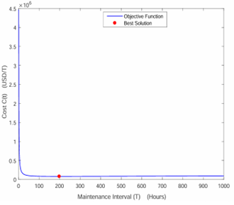
Table 2 indicates that performing maintenance on Conveyor No. 1 every 197.86 hours (or about every 8.24 days) will result in the lowest possible maintenance cost of 81,345.84 USD per time period. This optimized schedule helps in minimizing downtime and maximizing the efficiency and cost-effectiveness of the maintenance operations. Figure 1 graphically shows the evolution of cost C as a function of T.
The graph illustrates the relationship between maintenance periodicity (T) and the corresponding cost (C(T)). The curve rapidly decreases as T increases, indicating that frequent maintenance (low T values) incurs extremely high costs. As T increases, the cost drops sharply and then levels off. The red dot marks the optimal maintenance interval (T*), approximately 197.86 hours, where the cost is minimized. This optimal point highlights that very frequent maintenance is costly due to unnecessary downtime and labor, while infrequent maintenance increases operational costs and potential equipment failures. Thus, the graph emphasizes the importance of selecting the optimal maintenance interval to balance the frequency of activities with associated costs, ensuring a cost-effective maintenance strategy.
Figure 1. Objective function value vs. periodicity (T) for conveyor No. 1
3.1 ACO algorithm
ACO is an optimization technique inspired by the foraging behavior of ant colonies, first introduced by Marco Dorigo in the early 1990s. This algorithm mimics the way ants find the shortest paths to food sources using pheromone trails. Ants communicate and coordinate their actions through pheromones, which are chemical compounds secreted to create trails that guide other ants to food sources [18]. As ants travel, they deposit pheromones on the ground, which subsequently influence the path selection of other ants. The probability of following a particular path is higher if the pheromone concentration is higher, which leads to a reinforcement of shorter, more efficient paths as more ants follow and reinforce these trails. The evaporation of pheromones over time ensures that paths which are not frequently used gradually lose their attractiveness, thereby incorporating a mechanism for dynamic optimization. ACO has been effectively applied to a range of combinatorial optimization problems, such as the traveling salesman problem and network routing [19]. The algorithm's ability to adaptively find optimal solutions by simulating natural processes has made it a powerful tool in various fields of research and practical applications. The ACO algorithm is a robust tool designed for optimizing intricate problems, especially those with discrete or combinatorial search spaces. Its strength lies in its capacity to explore diverse solutions and iteratively refine them, guided by pheromone trails that encapsulate the collective wisdom of the ant colony.
When applied to the task of minimizing the objective function C(T), the ACO algorithm adeptly navigates through the solution space, constructing paths that lead to decreased values of C(T). Its efficacy hinges on several key parameters, including the number of ants, iterations, and rules governing pheromone updates. Below are the specific details of the ACO implementation:
Parameter Settings:
The fitness function for ACO is the same as the cost function C(T) derived in the study Eq. (10). The goal is to minimize C(T) by finding the optimal maintenance interval T∗.
Implementation Steps:
1) Initialize pheromone levels on all possible solutions (maintenance intervals).
2) Each ant constructs a solution (value of T) probabilistically based on pheromone levels and heuristic information.
3) Evaluate the fitness of each solution using the cost function C(T).
4) Update pheromone levels based on the quality of solutions found by the ants.
5) Repeat steps 2-4 for the specified number of iterations.
The accompanying MATLAB code offers a foundational framework for implementing the ACO algorithm tailored to specific problem requirements. Central to its application is the definition of the objective function C(T) and the customization of algorithmic parameters to align with the problem's nuances. By harnessing the ACO framework effectively, significant optimization gains can be realized across a broad spectrum of problem domains. The results of the program are gathered in Table 3.
Table 3. Results of ACO for conveyor system optimization
|
System |
Optimal Time (Hours) |
Optimal Time (Days) |
Min Cost (USD/t) |
Number of Iterations |
Execution Time |
Number of Evaluations |
|
Conveyor No. 1 |
196.374242 |
8.182260 |
81911.072031 |
28284 |
0.726214 seconds |
303800 |
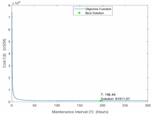
The results obtained using the ACO algorithm for Conveyor No. 1 reveal significant operational improvements. The algorithm pinpointed an optimal operational time of approximately 196.37 hours (8.18 days), striking a balance between productivity and resource utilization. This achievement is complemented by a minimal cost per unit time of 81,911.07 USD/t, indicating efficient economic management. The algorithm's performance metrics highlight its effectiveness: it converged after 28,284 iterations, executed in just 0.726214 seconds, and conducted 303,800 evaluations. These outcomes underscore ACO's capability in enhancing operational efficiency and cost-effectiveness in industrial settings, demonstrating its robustness in optimizing complex systems like Conveyor No. 1. Figure 2 graphically shows the evolution of cost C as a function of T.
Figure 2. Objective function vs. periodicity for conveyor No.1 optimized with ACO algorithm
The graph illustrates the relationship between operational period (T) and the corresponding cost C(T). The curve rapidly decreases as T increases, indicating that shorter operational periods (low T values) incur extremely high costs.
As T increases, the cost drops sharply and then levels off. The green dot marks the optimal operational period, approximately 196.38 hours, where the cost is minimized at 81911.07 USD/t. This optimal point highlights that very short operational periods are costly due to frequent stoppages and resource utilization, while excessively long periods can increase maintenance risks and potential equipment failures. This indicates that the optimal period represents the best trade-off between operational time and cost efficiency, achieving the most economical operation point. Additionally, the optimal period helps in scheduling maintenance more effectively, reducing the risk of unexpected breakdowns and ensuring smoother operations. By identifying this optimal period, the ACO algorithm aids in proactive maintenance planning, which can minimize downtime and enhance overall system reliability, thereby mitigating operational risks.
3.2 GA
GAs are powerful tools for optimization problems, widely used in various fields due to their ability to efficiently search through large and complex solution spaces. In the context of cost model optimization, GAs offers significant advantages by simulating the process of natural selection to identify optimal solutions that balance multiple competing objectives, such as cost, time, and resource utilization [20]. Below are the specific details of the GA implementation:
Parameter Settings:
The fitness function for GA is the same as the cost function C(T) derived in Eq. (10). The goal is to minimize C(T) by finding the optimal maintenance interval T∗.
Implementation Steps:
1) Generate an initial population of random solutions (values of T).
2) Evaluate the fitness of each solution using the cost function C(T).
3) Select parents for the next generation using tournament selection.
4) Perform two-point crossover on selected parents to produce offspring.
5) Apply Gaussian mutation to offspring to introduce diversity.
6) Replace the current population with the new generation.
7) Repeat steps 2-6 for the specified number of generations.
The MATLAB code for the GA, along with its associated subroutines, is already available. By simply programming the objective function and providing the failure and maintenance data, optimization results for this policy can be obtained. We have developed a MATLAB program to minimize our objective function C(T) using GA techniques. Table 4 presents the execution results.
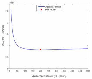
Table 4 provides key metrics and results from an optimization process related to Conveyor No. 1, detailing the time estimates, optimized performance metric (Cmin), and computational effort involved in achieving the optimization goals. Figure 3 graphically shows the evolution of cost C as a function of T.
Table 4. Results of ACO for conveyor No. 1
|
System |
T* in Hours |
T* in Days |
Cmin (USD/t) |
Number of Iterations |
Execution Time |
Number of Evaluations |
|
Conveyor No.1 |
197.8589 |
8.2441 |
81345.8372 |
200 |
1.897976 seconds |
20000 |
The Figure 3 illustrates the results of an optimization process using a GA, plotting the objective function value C(t) against periodicity T. The curve shows a steep decline in C(t) as T increases from 0 to around 100, after which it flattens out, indicating that further increases in T do not significantly improve C(t). The red dot on the curve marks the optimal periodicity found by the GA, around 197.8589, corresponding to the minimum C(t) of approximately 81345.8372. This point represents the most efficient periodicity for the system, balancing low objective function values with a practical periodicity, highlighting the GA's effectiveness in finding an optimal solution.
Figure 3. Objective function vs. periodicity for conveyor No. 1 optimized with GA
3.3 SA algorithm
SA is a probabilistic optimization algorithm inspired by the annealing process in metallurgy. Initially proposed by Kirkpatrick et al. in 1983, SA mimics the annealing process where a material is heated and then slowly cooled to achieve a more optimal state by minimizing defects and refining its structure [21]. This technique is particularly effective for solving complex optimization problems with large search spaces and numerous local optima. It starts with an initial solution and explores neighboring solutions, accepting not only better solutions but also, with decreasing probability, worse ones. This acceptance of worse solutions helps the algorithm escape local optima early on. The "temperature" parameter, which controls the acceptance probability of worse solutions, gradually decreases as the algorithm proceeds, reducing the search space and focusing on the most promising areas. This careful balance between exploration and refinement enables SA to effectively search for and identify optimal solutions in complex optimization problems. Below are the specific details of the SA implementation:
Parameter Settings:
The fitness function for SA is the same as the cost function C(T) derived in the study Eq. (10). The goal is to minimize C(T) by finding the optimal maintenance interval T∗.
Implementation Steps:
1) Start with an initial solution (random value of T) and set the initial temperature.
2) Evaluate the fitness of the current solution using the cost function C(T).
3) Generate a neighboring solution by perturbing the current solution.
4) Accept the new solution if it improves the fitness. If not, accept it with a probability based on the current temperature and the difference in fitness.
5) Reduce the temperature according to the cooling schedule.
6) Repeat steps 2-5 until the stopping criterion is met.
Here are the results obtained from implementing a MATLAB program using the SA algorithm we developed. The collected data provide a detailed analysis of the performance and improvements brought by our algorithmic approach.
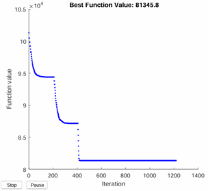
Table 5 presents performance metrics for Conveyor No.1 optimization using a SA algorithm. The optimal temperature parameter (T*) was determined to be approximately 197.8587 hours or about 8.182260 days. The algorithm executed 1280 iterations, with an execution time of 7.821692 seconds, involving 1280 evaluations. These results indicate that the SA approach effectively optimized the parameters for Conveyor No.1, achieving a significant reduction in cost while maintaining computational efficiency within a short runtime. Figure 4 graphically shows the evolution of cost C as a function of T.
Table 5. Results of SA algorithm for conveyor system optimization
|
System |
T* in Hours |
T* in Days |
Cmin (USD/t) |
Number of Iterations |
Execution Time |
Number of Evaluations |
|
Conveyor No.1 |
197.8587 |
8.182260 |
81345.8372 |
1280 |
7.821692 seconds |
1280 |
Figure 4. Objective function vs. periodicity for conveyor No. 1 optimized with SA algorithm
The graph showcases the relationship between maintenance periodicity (T) and cost (C(T)) as optimized by a SA algorithm. The curve's initial plunge reflects efficient exploration, identifying solutions with lower costs compared to frequent maintenance. As T increases, the cost levels off, signifying a shift towards exploiting promising areas. The red dot (T*≈197.8587) marks the optimal maintenance interval identified by the algorithm, minimizing cost (C(T)≈81345.8372 USD/t). This sweet spot balances avoiding unnecessary downtime and labor (low T) with minimizing equipment failures and operational costs (high T), highlighting the importance of selecting the optimal frequency for a cost-effective maintenance strategy.
To determine which optimization method is most effective for improving PM interventions, we will compare the performance of SA, GA, and ACO. This comparison will consider several factors, including the optimal maintenance interval (T*), minimum cost per ton (Cmin), number of iterations, execution time, and number of evaluations for Conveyor No. 1. By analyzing these metrics, we aim to identify the strengths and weaknesses of each algorithm in terms of accuracy, efficiency, and computational demand, providing insights into which method offers the best balance for enhancing PM strategies.
Table 6 provides a general comparison of three optimization methods-SA, GA, and ACO-for improving PM interventions on Conveyor No. 1. The exact mathematical calculation serves as a benchmark with an optimal maintenance interval (T*) of 197.86 hours (8.24 days) and a minimum cost (Cmin) of 81,345.84 USD/t. The exact Calculation presented in Table 6 represents the optimal solution obtained through a brute-force enumeration method. This approach systematically evaluates all possible maintenance schedules within the defined constraints. Specifically, for Conveyor No. 1, we generated and evaluated every possible combination of maintenance intervals, considering the underlying assumptions of minimal repair after failure and a Weibull distribution for system failure (γ=0). The cost function (Cmin) was calculated for each schedule, and the schedule that yielded the minimum cost was identified as the optimal solution. This exhaustive search method serves as a benchmark to assess the performance and accuracy of the heuristic optimization algorithms (ACO, GA, SA). Due to the computational complexity of brute-force enumeration, this method is only feasible for relatively small-scale problems, such as the single conveyor system considered in this study. The optimization algorithms used in this study ACO, GA, and SA each have distinct strengths and weaknesses. ACO excels in exploring complex search spaces and escaping local optima through pheromone trails but is computationally expensive and sensitive to parameter choices. GA is robust and effective for global optimization, maintaining diversity through crossover and mutation, but it can be computationally intensive and prone to premature convergence if parameters are poorly tuned. SA is simple to implement and computationally efficient, with the ability to escape local optima by accepting worse solutions early in the search, but its performance depends heavily on the cooling schedule and may not explore the search space as thoroughly as ACO or GA. While ACO and GA are better suited for global exploration, SA is more efficient for local refinement. These trade-offs highlight the importance of selecting the appropriate algorithm based on problem complexity, computational resources, and desired outcomes.
Table 6. Comparison of optimization algorithms for Conveyor No. 1
|
System |
Algorithm Used |
T* in Hours |
T* in Days |
Cmin (USD/t) |
Number of Iterations |
Execution Time |
Number of Evaluations |
|
Conveyor No. 1 |
Exact Calculation |
197.8589 |
8.2441 |
81,345.8372 |
/ |
/ |
/ |
|
ACO |
196.3742 |
8.1823 |
81911.0720 |
28284 |
0.7262 seconds |
303800 |
|
|
GA |
197.8589 |
8.2441 |
81345.8372 |
200 |
1.8980 seconds |
20000 |
|
|
SA |
197.8587 |
8.2441 |
81345.8372 |
1280 |
7.8217 seconds |
1280 |
In terms of performance, ACO achieved a similar T* but had a slightly higher cost and required many iterations and evaluations, showing high computational demand but quick execution. GA matched the benchmark precisely with fewer iterations and moderate computational resources. SA also matched the benchmark but was less efficient, needing more iterations and longer execution time. Overall, GA and ACO show strong performance in terms of accuracy and efficiency. For the number of objective function evaluations, ACO performs the most (303800), contributing to better exploration of the search space, while the GA performs 20000 evaluations, sufficient to reach an optimal solution efficiently, while SA, though accurate, is more time-consuming.
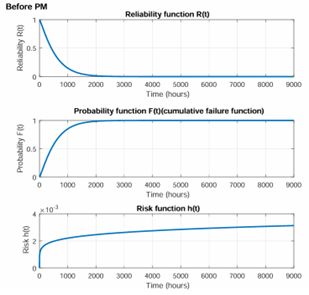
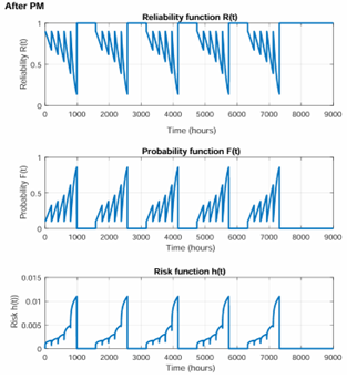
Optimizing PM using advanced methods is crucial for enhancing the systems reliability and industrial security. By implementing sophisticated techniques such as GA, SA, and ACO, industries can significantly improve the precision and efficiency of their maintenance schedules. These methods not only ensure that maintenance tasks are performed at optimal times but also contribute to reducing the likelihood of unexpected failures, thereby increasing system reliability and security. The following figure clearly illustrates the reliability graphs, the risk function, and the failure function after maintenance, providing a comprehensive overview of how these advanced methods positively impact industrial system performance.
Figure 5 illustrates the impact of a periodic PM strategy on system reliability, cumulative failure probability, and hazard rate. The reliability function R(t) exhibits a distinct, reflecting alternating phases of degradation and restoration. The downward slopes of the curve correspond to the natural decline in reliability between maintenance intervals, while the sharp upward jumps signify the restoration of reliability following PM interventions, effectively reducing the risk of system failure and maintaining a non-zero reliability value. Similarly, the cumulative failure function F(t) displays an inverse sawtooth pattern, with a gradual increase in failure probability during operational periods, followed by significant reductions after maintenance actions. This highlights the effective resetting of the failure probability by PM.
Figure 5. Graphs of reliability, risk function and failure function
The hazard rate h(t) further underscores the effectiveness of the PM strategy, exhibiting a cyclical trend characterized by a gradual rise in failure risk during system operation and abrupt declines immediately after maintenance activities. The periodicity of these cycles, observed at intervals of approximately 1500-2000 hours, defines the maintenance schedule and indicates the strategic timing of interventions. Overall, this analysis demonstrates that the PM strategy effectively mitigates the instantaneous risk of failure, sustains system reliability, and addresses degradation mechanisms or replaces critical components before catastrophic failure occurs.
In an industrial context, the application of optimization techniques and appropriate maintenance strategies is essential in enhancing the system's reliability and industrial security, ensuring the proper functioning and availability of equipment. The conclusions drawn from conducted studies provide valuable insights into the advantages and trade-offs associated with different approaches.
The analysis of optimization algorithms highlights the strengths and weaknesses of each method. GA and SA stand out for their precision and ability to converge to high-quality solutions, while ACO offers notable execution speed. This diversity of approaches allows practitioners to choose the method best suited to their specific needs, depending on time and precision constraints.
Regarding maintenance, the study emphasizes the importance of meticulous planning of periodic overhauls. The recommendation of partial overhauls after a certain number of operating days and a general overhaul after a longer interval is a wise strategy to maintain equipment reliability while minimizing downtime. Additionally, coordinating maintenance operations with other system components optimizes work efficiency and reduces production interruptions.
In the context of optimizing PM, advanced methods play a critical role in enhancing the system's reliability and industrial security. Techniques such as GA, SA, and ACO allow for precise scheduling and execution of maintenance tasks, reducing the likelihood of unexpected failures and ensuring continuous operation. These methods not only improve reliability but also contribute to the overall security of the systems by addressing potential vulnerabilities through well-timed maintenance activities.
In summary, these conclusions highlight the importance of optimization and planning in the industrial field. By adopting best practices and leveraging available optimization technologies, companies can improve their operational efficiency, reduce maintenance costs, and ensure optimal performance of their equipment.
To further advance the field of maintenance optimization, several research directions can be explored. Real-time data analytics could be investigated to enable continuous monitoring of equipment performance, allowing for predictive maintenance and just-in-time interventions. Sustainability integration should be prioritized, expanding optimization techniques to include environmental factors and aligning maintenance strategies with corporate social responsibility goals. Scalability studies are needed to explore the application of optimization algorithms to larger, more complex industrial systems with multiple interdependent components. Additionally, hybrid optimization models that combine the strengths of ACO, GA, and SA could be developed to achieve better performance across diverse industrial scenarios. Finally, human factor integration should be considered to incorporate decision-making processes and practical constraints into optimization models, improving their adoption and effectiveness in real-world settings. These research directions aim to enhance the applicability, efficiency, and sustainability of maintenance optimization in industrial environments.
|
Cc |
Corrective maintenance cost per year in Killo-United States dollar (KUSD/Y) |
|
Cp |
PM cost per year in Killo-United States dollar (KUSD/Y). |
|
Cov |
General overhaul cost per year in Killo- United States dollar (KUSD/Y). |
|
T |
Time (Hours or Days) |
|
H(T) |
Failure probability function |
|
C(T) |
Average cost per unit time. Killo-United States dollar per year (KUSD/Y). |
|
K |
Number of partial overhauls before the general overhaul |
|
n |
Total number of maintenance activities or interventions over a period |
|
Greek symbols |
|
|
a |
Maintenance efficiency factor, indicating the effectiveness of maintenance activities. |
|
b |
The degradation rate or other relevant factors. |
|
η |
The scale parameter of the Weibull distribution, representing the characteristic life. |
|
eα |
Degradation factor (exponential effect of degradation) |
|
Subscripts |
|
|
T* |
Optimal maintenance interval that minimizes cost |
|
c |
Corrective maintenance (related to repair cost) |
|
P |
PM (related to partial overhaul cost) |
|
ov |
General overhaul (full maintenance cost) |
[1] Wang, J., Miao, Y., Yi, Y., Huang, D. (2021). An imperfect age-based and condition-based opportunistic maintenance model for a two-unit series system. Computers & Industrial Engineering, 160: 107583. https://doi.org/10.1016/j.cie.2021.107583
[2] Pereira, C.M., Lapa, C.M., Mol, A.C., Da Luz, A.F. (2010). A particle swarm optimization (PSO) approach for non-periodic preventive maintenance scheduling programming. Progress in Nuclear Energy, 52(8): 710-714. https://doi.org/10.1016/j.pnucene.2010.04.009
[3] Kamel, G., Aly, M.F., Mohib, A., Afefy, I.H. (2020). Optimization of a multilevel integrated preventive maintenance scheduling mathematical model using genetic algorithm. International Journal of Management Science and Engineering Management, 15(4): 247-257. https://doi.org/10.1080/17509653.2020.1726834
[4] Fitri, L., Alhilman, J., Anggana, H.D. (2019). Optimization of machine preventive maintenance scheduling using steady state genetic algorithm. In International Conference on Rural Development and Entrepreneurship, Yogyakarta, Indonesia, pp. 525-534.
[5] Pandey, M.K. (2014). Selective maintenance for systems under imperfect maintenance policy. ERA. https://doi.org/10.7939/R3XP6V96P
[6] Wu, Z., Liu, B., Wang, Z., Ma, S., Ni, G. (2017). Research on condition-Based maintenance approach of power system considering equipment imperfect maintenance model. In 2017 Chinese Automation Congress (CAC), Jinan, China, pp. 3695-3700. https://doi.org/10.1109/CAC.2017.8243422
[7] Wang, J., Makis, V., Zhao, X. (2019). Optimal condition-based and age-based opportunistic maintenance policy for a two-unit series system. Computers & Industrial Engineering, 134, 1-10. https://doi.org/10.1016/j.cie.2019.05.020
[8] Jardine, A.K., Lin, D., Banjevic, D. (2006). A review on machinery diagnostics and prognostics implementing condition-based maintenance. Mechanical Systems and Signal Processing, 20(7): 1483-1510. https://doi.org/10.1016/j.ymssp.2005.09.012
[9] Hu, J., Jiang, Z., Liao, H. (2017). Preventive maintenance of a single machine system working under piecewise constant operating condition. Reliability Engineering & System Safety, 168: 105-115. https://doi.org/10.1016/j.ress.2017.05.014
[10] Alhourani, F., Essila, J., Farkas, B. (2023). Preventive maintenance planning considering machines’ reliability using group technology. Journal of Quality in Maintenance Engineering, 29(1): 136-154. https://doi.org/10.1108/JQME-12-2019-0118.
[11] Abdelhadi, A., Alwan, L.C., Yue, X. (2015). Managing storeroom operations using cluster-based preventative maintenance. Journal of Quality in Maintenance Engineering, 21(2): 154-170. https://doi.org/10.1108/JQME-10-2013-0066
[12] Li, X., Liu, Y., Han, Z., Chen, G. (2024). A risk-Based maintenance decision model for subsea pipeline considering pitting corrosion growth. Process Safety and Environmental Protection, 184: 1306-1317. https://doi.org/10.1016/j.psep.2024.02.072.
[13] De-León-Escobedo, D. (2023). Risk-based maintenance time for oil and gas steel pipelines under corrosion including uncertainty on the corrosion rate and consequence-based target reliability. International Journal of Pressure Vessels and Piping, 203: 104927. https://doi.org/10.1016/j.ijpvp.2023.104927
[14] Sin, I.H., Do Chung, B. (2020). Bi-objective optimization approach for energy aware scheduling considering electricity cost and preventive maintenance using genetic algorithm. Journal of Cleaner Production, 244: 118869. https://doi.org/10.1016/j.jclepro.2019.118869
[15] Huang, J., Wang, L., Jiang, Z. (2020). A method combining rules with genetic algorithm for minimizing makespan on a batch processing machine with preventive maintenance. International Journal of Production Research, 58(13): 4086-4102. https://doi.org/10.1080/00207543.2019.1641643
[16] Mobley, R.K. (2002). An Introduction to Predictive Maintenance. Elsevier. https://doi.org/10.1016/B978-0-7506-7531-4.X5000-3
[17] Tennant-Smith, J. (1978). Models of preventive maintenance. Journal of the Royal Statistical Society. Series C (Applied Statistics), 27(1): 85. https://doi.org/10.2307/2346238
[18] Rinne, H. (2008). The Weibull Distribution: A Handbook. Chapman and Hall/CRC. https://doi.org/10.1201/9781420087444
[19] Dorigo, M., Blum, C. (2005). Ant colony optimization theory: A survey. Theoretical Computer Science, 344(2-3): 243-278. https://doi.org/10.1016/j.tcs.2005.05.020
[20] Nayyar, A., Singh, R. (2016). Ant colony optimization-computational swarm intelligence technique. In 2016 3rd International Conference on Computing for Sustainable Global Development (INDIACom), New Delhi, India, IEEE, pp. 1493-1499.
[21] Shapiro, J. (1999). Genetic algorithms in machine learning. In Advanced Course on Artificial Intelligence. Berlin, Heidelberg: Springer Berlin Heidelberg, pp. 146-168. https://doi.org/10.1007/3-540-44673-7_7