Ehab Fakhri Hadi*![]() | Mohd Zafri bin Baharuddin
| Mohd Zafri bin Baharuddin![]() | Ahmad Wafi Mahmood Zuhdi
| Ahmad Wafi Mahmood Zuhdi![]() | Ghadir Kamil Ghadir
| Ghadir Kamil Ghadir![]() | Hayder Musaad Al-Tmimi
| Hayder Musaad Al-Tmimi![]() | Mohammed Ahmed Mustafa
| Mohammed Ahmed Mustafa![]()
© 2024 The authors. This article is published by IIETA and is licensed under the CC BY 4.0 license (http://creativecommons.org/licenses/by/4.0/).
OPEN ACCESS
In the field of predictive maintenance, accurately predicting the remaining useful life (RUL) of equipment is critical to optimizing operations and avoiding unexpected failures. Traditional models such as Gaussian Process Regression (GPR), Particle Filter (PF), and Kalman Filter (KF) have been widely used, each with their own strengths and limitations. The motivation behind this study stems from the need to improve the accuracy and reliability of RUL predictions. Given the critical importance of predictive maintenance across a variety of industries, improved predictive models can provide significant operational and economic benefits. The main issues addressed are the limitations inherent in individual predictive models. GPR prediction gap or high initial error of his KF. This can lead to suboptimal RUL estimates. To address this problem, an integrated approach combining particle filtering and Gaussian process regression (PF-GPR) was proposed and developed. This integration aims to leverage the strengths of PF and GPR and potentially alleviate the limitations of the individual models. The performance of the PF-GPR model is evaluated and compared with the standalone His GPR, PF, and KF models using the prediction error and root mean square error (RMSE) at different points in the aging process of device #36. The results show that the PF-GPR model consistently outperforms the individual models in terms of both prediction error and RMSE, and significantly improves the accuracy and accuracy of RUL prediction. The PF-GPR model showed excellent performance in his RUL prediction for device #36, achieving the lowest prediction error and RMSE values at all time points as follows: B. The prediction error is only 2.30E-1 and the RMSE after 100 minutes is 7. 12E-3, which significantly outperforms his standalone GPR, PF, and KF models. The PF-GPR model demonstrated its excellent ability to provide robust and reliable predictions, highlighting the benefits of integrating different prediction methods into predictive maintenance applications.
electronic medical record, blockchain technology, NSGA-II, NSGA-III, hyper-volume
Electric devices with silicon at their heart, namely the metal-oxide-semiconductor field-effect transistors (MOSFETs) and the insulated-gate bipolar transistors (IGBTs), are extensively embraced in the power electronics field for examples electricity conversion, renewable energy generation, and transport energy applications. FASIT technology won't be without MOSFET power, renewable energy including radio frequencies and vibration helps innovative power generation solutions and improved device optimization, green vehicles (sp) and hybrid vehicles. The consumption of power that is associated with microprocessors, mobile devices, and health electronics is one of the harshest power-problems that we face today. Reliability, however, is of the paramount significance, since even the most minor failure can lead to chain of serious disruptions or a system shutdown. With that being said, one of the most significant advantages precisely becomes prognostics that are the ability damage levels monitoring and predictive maintenance. This function of prophesy allows discovering faults beforehand so that a piece of seldom-used machinery can be either repaired or substituted for some appropriate device. Consequently, this not only guarantees the perfect functioning of the systems, but the goal of lifetime extension as well. The savings in costs will thereby be a found outcome.
Metal-Oxide-Semiconductor Field-Effect Transistors (MOSFETs) are indelible key in modern electronics and applications; they determine the future of the industry we know today. The features that differentiate these devices, like clock speed lower than normal, well-spent energy, and instant switching on/off, make them useful in various sectors. MOSFETs have are a major factor in designing and management of solar inverters and wind turbine controllers in the renewable energy sector. These apparatuses convert the DC from solar systems and wind generators into AC, making possible the establishment of growing renewable generating sources in the grid. Both MOSFET and power-electronics enable modernization of power systems and renewable integration programs, which fare on the shoulder of the implementation of sustainable energy solutions [1].
That on one hand, the automotive industry also gets lot of benefits because of MOSFET technology especially for electric vehicles (EV) and hybrid automobiles (HV). MOSFETs as well as numerous subsystems including battery management system (BMS), DC/DC converters and motor drives are widely used. Their effectiveness in power conversion as well as the capability of operating at high frequency creates MOSFETs the most suitable for this job ensuring best vehicle performance, longer battery life and lesser energy losses [2].
MOSFETs find wide application in power management area of design of power supply unit (PSU) components for consumer electronics, machines for communication and industrial processes. They regulate voltage and current to provide momentary power delivery, without which the lifespan of the majority of precision and electronic devices would matter little. The energy efficiency of MOSFETs offers not only their conservation benefits but they are also used to prolong the life of electronic devices through reduced generation of heat. MOSFETs are widely used in newer communication systems as the frequency goes higher and higher ones such as radar, satellite, and radio communication. Their operation with high efficiency on a relatively wide range of frequencies for amplification and switching jobs gives them credibility in communication in complex systems that cover vast distances, clarity among others [3].
In the healthcare sector, MOSFETs are incorporated in multiple medical devices such as portable diagnostic tools, monitoring of patients and surgical machineries. These devices have a simple, yet deterministic control of the power which is vital for systems utilized in exact procedures to achieve patient security and to improve the effectiveness of the medical procedures [4].
The MOSFETs are used everywhere from Smartphones to laptops at home appliances and gaming consoles. Devices in IoT use less energy because of the effective power management method and its capacity to have small designs, longer battery life, and high-end performance. Since the dawn of MOSFETs in Consumer Electronics, technology has signified the revolution and progress in the industries with regards to user experience as well as device capabilities due to the increase in the capabilities of devices [5].
MOSFETs are indispensable components in motor control and drive systems whether industrial automation and robotics is concerned. They provide smooth motions control between speed, torque, and position of a motor which is used in the production automation systems (i.e., robotic arms and conveyor systems). In this context, MOSFETs will greatly improve efficiency and reliability, help to decrease power consumption and effectively regulate the processes of smart manufacturing thus advancing the industry [6].
ON-state resistance which has been applied as the major qualitative indicator of fault in binomial and data-driven prognostic algorithms in previous studies. The study of device deterioration is one significant area of power electronics where data-driven or AI techniques find use. Power devices have a lengthy life span in some applications, and it may take years for them to malfunction or degrade. However, collecting, storing, and analyzing such a large dataset to examine the degrading attributes or lifetime of power devices is not practical. This is accomplished through accelerated testing, in which the device is subjected to various sorts of stressors (thermal or electric) in order to speed up the device's degradation. In such accelerated tests, a failure precursor is identified first, and the sensor data collected during the test is analyzed using model-based and/or data-driven approaches to anticipate the time to failure (TTF), remaining useful life (RUL) of the power devices [7].
Failure of these devices is often associated with increased on-state resistance, which can be caused by a variety of factors, including wire bond degradation, gate oxide defects, and chip attachment cracks and delamination’s. There is a gender. However, on-state resistance is not the only characteristic used to diagnose the condition of a MOSFET.
Another important property is breakdown voltage. Changes in breakdown voltage can indicate potential problems with your device. Interface recession problems or hot carrier effects. In order to develop brighter, more energy-efficient lights, critical issues related to semiconductor materials must be addressed, including interfacial recession issues and hot carrier effects. Through these measures, predictions go into the health of your system very significant and useful. Besides, employing the pre-diction may add up to the increasing efficiency of scientific equipment. It is critical that the knowledge gain of the underlying factors of and failure patterns arising from evolving equipment assists manufacturers in enhancing the design and production processes for this equipment which increases their efficiency and reliability [8].
Modern prediction models although particular for the prediction of Remaining Useful Life (RUL) have some limitations when they are asked to predict the MOSFETs [5], because these models are complex in nature.
What causes problems is the brittleness of the concepts arising from the inability of these models to translate the complicated and non-linear nature of the behavior of any MOSFET device under varied conditions to electronic effects. The conventional approaches, majority of which obey the linear and static paradigms, fall short of grasping the complex MOSFET deterioration phenomenon which is subject to variety of stimuli including thermal cycling, electrical tension overload, and mechanical exposure [9].
The problem could worsen due to the fact that models are majorly dependent on failure data of traditional processing technologies whose data could not be found for emerging technologies faster and may also become quickly irrelevant due to the rate of innovations in semiconductor devices. For instance, these models are not good at dealing with breakthrough failures that appear only in rare cases, while paying major attention to usual degradation reasons and in the process passing up less probable breakdowns not considered catastrophic. Then, generalization becomes even more problematic when it comes to porting these models across various types of MOSFETs and their applications, individually exhibiting specific operational stresses and necessities following specific requirements [10].
However, the introduction of these challenges means that there is a great need to move to data-driven algorithms, particularly those ones use the ML and DL, which are a big strides in technology. Such approaches are superior to their competitors in making use of the available datasets, adapting to the complex degradation patterns, and in the prediction, which is of the greatest importance, of RUL [11, 12].
The integration of AI/ML with classical filtering methods such as the Kalman or the particle filtering is such that not only do the predictive accuracy moves up but also the adaptiveness and the reliability of the RUL estimation in the monitoring of sophisticated MOSFET applications takes center stage thereby ushering in a new era in power semiconductor devices prognostics [13].
In many areas of security, healthcare, and the like, ML technologies are becoming more attractive, including numerous mathematical models [14, 15], and deep learning (DI) that may revolutionize the way in which we use smart phones, TV, and cars. as a result of growing data amounts and innovative deep learning (DL) tech, there can be deep learning (DL) approaches considered to boost graphs [16, 17].
However, a fundamental challenge in applying ML/DL algorithms is their reliance on large-scale training data, which is not always readily available. Additionally, developing predictive models that can be universally applied to a variety of devices has proven inefficient due to the inherent differences in manufacturing processes and environmental influences for each device.
Instead, statistical filtering techniques such as Kalman filtering and particle filtering have proven to be promising approaches. Particle filtering is used in visual tracking, navigation, and guidance, automatic control, signal processing, fault diagnosis, and analysis [18]. Kalman filter algorithm is a model-dependent method that provides true-time forecasts using a mistake correction technique. These methods have the advantage of not requiring large datasets for effective model building. It also has real-time operational capabilities, making it suitable for predictive applications [19, 20].
However, these methods rely on models trained on short-term data and lack a long-term perspective on device behavior, which limits their long-term predictive capabilities.
A notable gap in current literature is the integration of ML/DL and statistical filtering methodologies. Such a synergistic approach could potentially address the constraints of each method individually. By combining the advanced pattern recognition and predictive power of ML/DL with the real-time processing and lower data requirements of statistical filtering methods, it is conceivable to enhance the accuracy and reliability of prognostics. This integrated approach could provide a more comprehensive understanding of device behavior over longer periods, which is crucial for effective maintenance and operation in power semiconductor devices.
This article aims at performing MOSFET prognostic using ON-state resistance as precursor variable based on an innovative integration between statistical filtering, namely, particle filtering with famous machine learning method, namely, Gaussian regression process.
The proposed integration is proposed for complementary long-term perspective of Gaussian regression process with short term perspective of particle filtering. The remaining of the article is organized as follows. In section 2, we present the contributions. Next, the related works are presented in section 3. Afterwards, the methodology is presented in section 4. Next, the experimental results and analysis are presented in section 5. Finally, the conclusion and future works are presented in section 6.
This article aims at proposing a novel MOSFET prognostic using combination between particle filtering and Gaussian regression process. The article presents several contributions to the literature, they can be stated as follows.
(1) To the best of our knowledge, this article is the first that addresses the problem of MOSFET prognostic using forecasting approach. It provides not only calculation of the deviation between forecasted values of the precursor variable and the true values but also it provides calculation of the prognostic error which is the difference between the true failure point of time and the predicted one.
(2) It provides a novel framework that combines particle filtering (one type of statistical filtering) with Gaussian regression process (one type of machine learning methods). Such framework enables complementing the long term perspective of trained model with short term perspective of statistical filtering making it as effective solution for MOSFET prognostic.
(3) It provides thorough evaluation of the proposed approach and comparison with various state of the art algorithm demonstrating its capability of handling prognostic in the situation of data shortage.
This section deals with the Litturature review of the prediction methods of MOSFET reliability. Among them two sub-sections made of beds positioned closely together. To the first, we shall among the related works of MOSFET reliability and its typical problems are put. Following the MOSFET MTS, another method is described in section 3.
3.1 Related works
Reliability and longevity concerns for metal-oxide-semiconductor field-effect transistors (MOSFETs) play a crucial role in power electrics, MOSFETs, which nowadays perform such a special duty as managing power conversion and control tasks various applications. This section discusses normally expected MOSFET performance degradation problems, together with a number of proposed (in the literature) remedies to tackle these shortcomings.
Identifying the remaining useful life (RUL) accuracy of MOSFETs is a challenge caused by signal noise in degradation data and variability threshold for failures among individual devices. These fluctuations therefore do not facilitate the precise evaluation of the flavor of the MOS monocrystal, as well as the forecasting its LEL. Zhao et al. [21] promote the Gamma state-space model application for the degradation model uncertainty mitigation: temporal, seed-to-seed, and device-to-device heterogeneity), by means of the stochastic expectation-maximization algorithm for parameter estimation [22]. Moreover, it uses a nonlinear Wiener process, which includes the estimation of the failure threshold uncertainty, with the help of a normal distribution truncated to account for the device diversity in the RUL estimation performance. The unsteady or invisible breakdown law of MOSFETs as well as relevant elements makes it difficult to practice the conventional model-based approaches for RUL prediction, which exacerbates the problem of precise time-to-death estimation.
Al-Mohamad et al. [23] adopt a coupled process and path-independent prognostic approach without taking any knowledge about past degradation profile of the system. The AJEKF is used inside the framework for the parameter estimation and degradation forecasting. Ibrahim et al. [24] learn prognostic modelling based on degradation data and using LSTM and GRU algorithms, which employs effective predictions engine and error correction mechanism, achieving better results than traditional ones [24]. Integrating physical knowledge, reliability data, and real-time operational data to improve RUL estimation accuracy is a complex challenge due to the diverse nature and sources of these data types. Djeziri et al. [25] use physical models to link reliability test features to variables measurable online, generating health indices for RUL estimation and updating these models based on online data. Ren et al. [26] combine LSTM networks with optimization techniques for improved prediction accuracy, indicating a methodological shift towards data-driven approaches.
MOSFETs operate under a wide range of conditions, making it challenging to predict their RUL due to changing stress levels, temperatures, and operational cycles. Sayed et al. [27] propose a statistical approach using probability density functions based on experimental degradation data for real-time RUL prediction of GaN-based converter systems, reflecting the method's adaptability to different operational profiles. Kathribail and Vijayakumar [28] conduct a comprehensive study of MOSFET degradation and develops a prognostic failure detection method using physical models and case temperature as a precursor, catering to early detection of MOSFET degradation.
Through the exploration of these common problems and the diverse methodological approaches proposed in the literature, this survey highlights the multifaceted challenges in MOSFET reliability research. The solutions presented, which begin with smart data-driven modeling and proceed to adaptive filtering techniques and singularity permutation and physical analysis bear the most practical significance in the advancement of the field, the aim of which is to improve the accuracy and reliability of these crucial components. Prognostic methods for MOSFET are being the next section which are basing on machine learning or statistic filtering.
3.2 MOSFET prognostic
Research in MOSFETs prognostic has seen the merge of machine learning and aspects data-centric to boost the accuracy of the prediction and the reliability of it. Celaya et al. [29] have the emphasis on the balance of two formulas for prognosis of service life in MOSFET semiconductors. They teamed reliability data–based with hardware model–based methods in their prognostics research. They discovered that the observed end-of-life failure mode was inter-acid barrier die-attach degradation, and with ON-state resistance being the affected component exhibiting a rise due to high thermal stresses. They look at the use of the Gaussian process regression algorithm in model-free techniques.
Ren et al. [26] effectuated a computer-aided way of life prediction on the thermal stress energy preservation of power MOSFETs. They have come to the conclusion that the ON-state resistance as a failure parameter precedent is the one that should be taken into account and together with the Autoregressive Integrated Moving Average (ARIMA) model, which is expressed in the data-driven way, should be used for life expectancy applying. Dash et al. [30] further demonstrated the RUL prediction model designed based on the features of the ANN. Their model utilized key time-domain features extracted from degradation profiles, which were selected based on their correlation with the target output. LSTM networks have been employed in several studies.
Bai et al. [31] combined the LSTM algorithm with the discrete hidden Markov model (DHMM) and an autoregressive (AR) model for feature extraction. In another study, Wu et al. [32] integrated LSTM with adaptive moment estimation algorithms, Dropout techniques, and Bayesian optimization methods.
Bai et al. [31] combined stress wave signals of the device with deep learning to determine the device's working state. Their approach utilized 1DCNN combined with time-domain series.
Alonso-González and Pulido [33] explored simpler techniques, such as least squares or horizontal average, within a Big Data platform. Their approach was compared with other techniques in the literature.
Sharma [34] conducted a study on MOSFET degradation, identifying ON resistance (${{R}_{DSon}}$) variation as a primary degradation parameter. They calculated power dissipation and subsequent junction temperature variation, using the measurable case temperature to design a detector for buck converter failure due to MOSFET degradation. Other contributions include the study of Ni et al. [35], who presented a Particle Filter method for predicting the remaining useful life of MOSFETs based on on-resistance (Ron) changing data, and Boutrous et al. [36], who used evolving fuzzy models and data-driven techniques for IGBTs. Upon careful examination of Table 1, which provides a comprehensive survey of existing research methods in the prognostics of Metal-Oxide-Semiconductor Field-Effect Transistors (MOSFETs), a variety of approaches emerge. These include statistical techniques like Gaussian Process Regression (GPR) and ARIMA, as well as machine learning strategies such as Long Short-Term Memory (LSTM) and Artificial Neural Networks (ANN). A common thread among most of these studies is the use of direct forecasting models to predict MOSFET malfunctions, with a particular focus on the ON-state resistance (${{R}_{DSon}}$) as a primary indicator.
However, a notable gap exists in the current research landscape: the data instability introduced by non-stationary time-series data, especially in cases of ${{R}_{DSon}}$scenario. Data are the crucial element of any forecasting model where the RDSonparameter is normally indicated as a steady though fluctuating variable over time. Utilization of this analysis method with different values of ${{R}_{DSon}}$may become the basis for wrong forecasts. The present gap in this research is telling of the need for improved prediction models that can cope with the complications that arise when dealing with non-stationary time-series datasets, such as ${{R}_{DSon}}$and RDSD day. Such a practical model would be using more reliable and accurate prediction tool which is very important factor to optimizing maintenance schedules, extending the period of MOSFET devices, and reducing the percentage of unpredicted failures.
The way ahead requires the identification of the pros of machine learning/deep learning and statistical filtering methods and developing means to combine their advantages. Machine learning and deep learning algorithms with the ability to process and interpret complex data patterns, as well as a statistical filtering view, which offers a narrow-focus detail on short-term prediction based on current states, are among the different approaches that are used in modern computational intelligence. Despite the fact that the solution is inevitable and possible, the combination of these methodologies is able to overcome the individual limitations of each approach and create more accurate, robust framework for MOSFET failures prediction. This model integration of MOSFET prognostics leads for a huge enhancement in the area known as MOSFET prediction, which in turn will help in making effective and efficient management of vital components.
Table 1. An overview of existing articles in MOSFET prognostic
|
No. |
Article |
Method |
Precursor |
Improvement |
Limitation |
|
1 |
[29] |
|
ON-state resistance |
Visualization only |
|
|
2 |
[37] |
ARIMA Guass newton iteration |
ON-state resistance |
Incorporation of assumed degradation model which implies simplification |
It is dependent on how much the degradation is accurate Tylor series implies losing of accuracy |
|
3 |
[30] |
Artificial neural networks (ANN) MLP |
Electrical component data |
Real world experiment |
Shallow learning which sufficiency in capturing huge data patterns |
|
4 |
[8] |
(LSTM) algorithm with the Discrete Hidden Markov Model (DHMM) With the aid of autoregression model |
ON-state resistance |
State health recognition using DHMM |
Lacking of sensitivity analysis of the failure threshold |
|
5 |
[26] |
Adam, Dropout and Bayesian algorithms are used to optimize LSTM |
ON-state resistance |
Optimization of LSTM |
Lacking of quantization of the performance results with respect to the variability of the AAT length |
|
6 |
[31] |
1-D convolutional neural network (1DCNN), long short-term memory (LSTM), and recurrent neural network (RNN) |
Acoustic emission signal |
1DCNN |
It can only distinguish the working state of the device, but the recog- nition effect of the device in different health states is still unclear |
|
7 |
[33] |
Model fitting |
ON-state resistance |
Linearization And least square error |
Not effective because of assumption of unique exponential model of the device and because of the error resulted from the linearization |
|
8 |
[34] |
Simulation using spice Physical model |
Tc temperature of the case |
Propose a new degradation model |
It does not have prediction of failure |
|
9 |
[32] |
Particle Filter algorithm with strong tracking Kalman filter (STKF) for weights updates and Metropolis–Hastings algorithm for resampling |
ON-state resistance |
Incorporate Kalman and Metropolis–Hastings algorithm inside Particle Filter |
The prediction results may be influenced by the linearization, with the STKF introduced into the PF |
This section presents the developed methodology. It starts with the problem formulation. Next, we present the Particle Filter framework.
4.1 Problem formulation
Assuming that we have a MOSFET device, and a time series of a precursor variable, namely, on-state resistance between drain and source ${{R}_{DS-on}}\left( t \right)$ after normalization. The goal is to build a prognostic model for the MOSFET based on ${{R}_{DS-on}}\left( t \right)$ from the start of the data ${{t}_{0}}$ until the prediction moment ${{t}_{p}},$ ${{R}_{DS-on}}\left( {{t}_{0}}:{{t}_{p}} \right)$ in order to minimize the prognostic error that is given by the Eq. (1).
$Erro{{r}_{prognostic}}=\left| {{{\hat{R}}}^{-1}}_{DS-on}\left( {{t}_{f}} \right)-{{R}^{-1}}_{DS-on}\left( {{t}_{f}} \right) \right|$ (1)
where,
${{R}^{-1}}_{DS-on}\left( {{t}_{f}} \right)$ denotes the inverse function of on-state resistance at the moment of failure, this indicates to the actual moment of failure ${{\hat{R}}^{-1}}_{DS-on}\left( {{t}_{f}} \right)$ denotes the inverse function of predicted on-state resistance at the moment of failure, this indicates to the predicted moment of failure.
The decision variable that is used to provide the error $Erro{{r}_{prognostic}}$ is mainly dependent on the mathematical model of predicting the on-state resistance ${{\hat{R}}^{-1}}_{DS-on}\left( {{t}_{f}} \right)$ in its inverse form.
4.2 Theoretical background
This subsection explains the theoretical background and the four conceptual models precisely required which will facilitate understanding of PF and GPR integration into the prognostic modeling of MOSFET devices. Such non-linear modeling strategies are, therefore, relevant to the process of reliable and precise life cycle of a part prediction.
4.2.1 Particle Filter (PF)
The Particle Filter performs as a strong tool for sequential state estimation in complex problems with nonlinear state space and non-Gaussians. It applies the technique, referred to as sequential importance sampling (SIS), which writes out the weighted sample vectors in the space of variables; the sample vectors are known as particles. Each particle is a type of state which may exist in the system and its weight is the calculation of likelihood of this state in view of that data being at hand. Through the following steps, LKC has implemented its PF system:
(1) Initialization: Give particles across the room the initial positions by means of a prior knowledge or a uniform distribution.
(2 Prediction: Instantiate and propagate individual particle of around the whole system which is accurate to the system than the dynamic model, and taking into account the noise.
(3) Update: Set particle weights in proportion to prospective errors of forthcoming observations, allowing seamless incorporation of new readings to the estimation scheme.
(4) Resampling: Solve the problem of degeneracy by re-weighting the particles and discarding those with weights lower than required for the simulation to be meaningful.
4.2.2 Gaussian Process Regression (GPR)
The generalized predictive modeling with prior regression is a non-parametric and Bayesian technique for regression application, which gives a flexible framework for data modeling. It clubs a function having a Gaussian process prior (which is then updated from a posterior) into the observed data. This approach has an outstanding let in making prediction with the estimation of uncertainties which is a classy element in predictive models that addresses the inherent random in the system behavior and uncertainties of the measurement process. GPR comprises: When students actively participate in group discussions or collaborate on projects, they are more likely to engage with course content and retain information for a longer period of time:
(1) Kernel Function: With its parameter capturing the covariance between points in the input space it provides a means of defining the smoothness, periodicity and other properties of the function being modeled thus allowing for expansion beyond linear regression. Choosing a the kernel is important in how model can perform its the task of data fitting and predicting on unknown.
(2) Training: Tat knowns as the kernel optimization, which consists of fine-tuning of the hyperparameters so that they can satisfactorily describe the observed data, usually by maximizing the likelihood of data on the model.
(3) Prediction: In addition to the point estimation, GPR gives out a predictive distribution (between mean and variance) for the underlying output function of a new input. This distribution tells about both the expected value of the given function for that particular point and the uncertainty namely the variance of the given point.
4.3 General algorithm
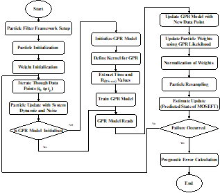
The flowchart is framed with an algorithm that captures the interplay of Particle Filter (PF) and Gaussian Process Regression (GPR) (Figure 1). It is in fact a predictive maintenance problem with the prediction of remaining useful life (RUL) of the equipment. The process beings with setting up the Particle Filter framework, at the beginning, the particles display probable system states.
While at the same time, the weights are initialized which is what will later serve as the basis of iteration. In the meantime, the Gaussian Process Regression model is established, and the kernel (the one that captures within the date correlation structure), is defined, and then the model is trained based on time and RUL data accumulated from historical data datasets.
After all, the algorithm authorizes the iterative stage to operate as the information is handled one item at a time. The next part of the algorithm involves, particle updating using the dynamic model and noise associated. If the output of GPR too close to the target data is not too far, the GPR model is ready, otherwise not. If not, it sends itself back to repeat, another loop running through numerous data points.
Once GPR model is ready, PF uses the resulting likelihood to update the particle weights, which in turn reflect the additional information that particles carry about the estimate that each one may depict. Then, it is followed with the biased introduction of weights normalization and the resampling that standard to both PF and PF to prevent degenecy and letting the machine focus on the more likely states.
Subsequently, the PF provides the result of the predicting algorithm. It presents an estimate about the current condition of a system component, for instance, a MOSFET. In case a fault is recognized, the execution breaks and then, the misclassification probe calculates the precision of the failure prediction. In the course of the mission, the GPR model is always the latest one to incorporate new data entries, thus, the tuning parameters can change in the PF framework.
This creates a feedback loop where both models are dynamically informed by the latest data, enhancing the accuracy and reliability of the RUL prediction. The process concludes with the final prognostic error calculation once a failure has occurred or the prediction task is complete.
Figure 1. Flowchart illustrating the procedural integration of Particle Filter and Gaussian Process Regression for remaining useful life prediction
4.4 Particle Filter framework for MOSFET prognostic prediction
In the pseudocode for a Particle Filter framework applied to the prognostics of MOSFETs given in Algorithm 1, the process begins with the inputs of the time series of normalized on-state resistance between drain and source ${{R}_{DS-on}}\left( t \right)$ at the start time of the data (${{t}_{0}}$), and the prediction moment (${{t}_{p}}$). The output aimed for is the estimated state of the MOSFET at the moment of failure.
The moment of failure is defined by the moment when ${{R}_{DS-on}}\left( t \right)$ cross the value 0.05.
Initially, particles are initialized, with each particle representing an estimate of the system state at the start time ${{t}_{0}}$. Following this, weights are assigned to each particle, usually beginning with equal weights for all. The weights are then reshaped as required.
During the whole process, the algorithm loops through the data atoms starting from the launch time range to the moment that the prediction is being made. At each time step, they are a composite of the device dynamics and the random evolution which they convey. The update now involves having at disposal the application of a model of MOSFET degradation and the inclusion of process uncertainty in form of noise. Parallel with that, the particles’ weights are updated in accordance with the probability of the$~{{R}_{DS-on}}\left( t \right)$ run observation at each step of time with a given state of the particle being the input. We need to proceed with the calculation of the probability of the particular state of the system corresponding to the given measurement. The dimensions are standardized with sum equal to one out of all elements, that guarantees correct relative probabilities.
Here the crux of the process resides: particles are resampled in accordance with the new weights, with the primary focus on the likely states. One of the main functions of this process, aside from compensating for particle depletion and providing a variety of particles, is to provide the correct frequency, phase, and amplitude within the filtered signal. This estimated final state replaces the constituent particles with weighted means of them, and it approximates the state of the MOSFET at the failure's current time.
Finally, the framework concludes with the calculation of prognostic error. This error is computed by comparing the inverse function of the actual on-state resistance at failure and the inverse function of the predicted on-state resistance at failure, thereby determining the accuracy of the prediction made by the Particle Filter framework.
Algorithm 1. Particle Filter framework for MOSFET prognostic model
|
Inputs: - ${{R}_{DS-on}}\left( t \right):$ Time series of normalized on-state resistance between drain and source as the measurement input. - ${{t}_{0}}$: Start time of the data. - ${{t}_{p}}$: Prediction moment. Outputs: ${{t}_{f}}$ the moment of failure ${{E}_{p}}$ Prognostic error Start: 1. Particle Initialization: Each particle is initialized to represent an estimate of the system's state, specifically ${{R}_{DS-on}}\left( t \right)$ at ${{t}_{0}}$. 2. Weight Initialization: An initial weight is assigned to each particle. Typically, these weights start equally. The weight array may be reshaped as required. 3. Data Point Iteration (From ${{t}_{0}}$ to ${{t}_{p}}$): The process iterates through each time step $t$ ${{R}_{DS-on}}({{t}_{0}}$ to ${{t}_{p}})$. 3.1. Particle Update with System Dynamics and Noise: The MOSFET degradation model is applied to each particle, integrating random noise to mimic process uncertainty. 3.2. Weight Update Based on Measurement Likelihood: Each particle's weight is recalculated based on the likelihood of the observed ${{R}_{DS-on}}\left( t \right)$, given the particle's state. This involves computing the probability of the measurement relative to the particle's predicted state. 3.3. Normalization of Weights: Weights are adjusted so their sum equals 1, preserving their relative probabilities. 3.4. Particle Resampling: Particles are resampled based on updated weights, focusing on more probable states, addressing particle depletion, and ensuring diversity. 3.5. Estimate Update: The final state estimate is computed as the weighted mean of all particles. This estimate represents the predicted state of the MOSFET. 3.6. Failure Moment Check: The state of the MOSFET is checked to determine if it has reached the moment of failure, specifically testing whether the predicted state equals 0.05. If this condition is met, the loop is terminated. 4. Prognostic Error Calculation: The prognostic error is computed by comparing the inverse function of the actual on-state resistance at failure with the inverse function of the predicted on-state resistance at failure. End |
4.5 Gaussian regression process
Gaussian Process Regression (GPR) is a powerful, non-parametric statistical modeling technique used in machine learning for making predictions about complex, unknown functions. The core concept of GPR is to place a Gaussian process prior over functions and use observed data to update this prior into a posterior over functions. The strength of GPR lies in its flexibility and ability to model complex datasets with relatively few assumptions about their underlying structure.
An exponential model for ${{R}_{DS-on}}\left( t \right)$can generally be represented as Eq. (2).
${{R}_{DS-on}}\left( t \right)=a{{e}^{bt}}+c$ (2)
where,$a$,$b$ and $c$ are parameters of the model. Here, $a$ represents the initial value of ${{R}_{DS-on}}(t$) at $t=0$, $b$ represents the rate of change of $RD\text{Son}$, and $c$ is the asymptotic value that $RD\text{Son}$ approaches as $t$ becomes large.
To fit this model using GPR, we first need to define the Kernel Function. The choice of kernel is critical. Given the nature of the exponential behavior, a kernel that can capture this trend should be used. A common choice might be the Rational Quadratic kernel or the Exponential kernel, which can model varying degrees of smoothness in the data. With dat $t,{{R}_{DSon}}\text{ }\!\!~\!\!\text{ }\left( t \right)$ we train the Gaussian Process by computing the covariance matrix using the kernel function for the training data. We use the GPR model to make predictions at new time points. The GPR will provide a mean prediction function which can be interpreted as the expected value of$\text{ }\!\!~\!\!\text{ }{{R}_{DSon}}\left( t \right)$ at each time point, along with a confidence interval that represents the uncertainty of the prediction. We present the pseudocode for prediction using GPR in Algorithm 2.
Algorithm 2. Pseudocode for predicting ${{\text{R}}_{\text{DSon}}}$ (t) using Gaussian regression process
|
Inputs: - ${{R}_{DSon}}$_data: Array of ${{R}_{DSon}}$ (t) data (time, ${{R}_{DSon}}$value pairs) - t_new: Time for new ${{R}_{DSon}}$prediction Outputs: - ${{R}_{DSon}}$_pred: Predicted ${{R}_{DSon}}$value at t_new Start: 1. Define Kernel for GPR: $kernel\left( t1,~t2 \right)~=~sigma\hat{\ }2~*~exp\left( -abs\left( t1~-~t2 \right)\hat{\ }2~/~\left( 2~*~length\_scale\hat{\ }2 \right) \right)$ 2. Initialize GPR Model: $GPR~=~GaussianProcessRegressor\left( kernel=kernel \right)$ 3. Extract Time and ${{R}_{DSon}}$Values from Data: $~~~t\_values~=~ExtractTimePoints\left( {{R}_{DSon}}\_data \right)$ $~~~{{R}_{DSon}}\_values~=~ExtractRDSonValues\left( {{R}_{DSon}}\_data \right)$ 4. Transform ${{R}_{DSon}}$Values: $~~~transformed\_{{R}_{DSon}}\_values~=~LogTransform\left( {{R}_{DSon}}\_values \right)$ 5. Train GPR Model: $~~~GPR.fit\left( t\_values,~transformed\_{{R}_{DSon}}\_values \right)$ 6. Predict Log-Transformed ${{R}_{DSon}}$at t_new: $~~~log\_{{R}_{DSon}}\_pred,~sigma~=~GPR.predict\left( t\_new \right)$ 7. Transform Prediction Back to Original Scale: $~~~{{R}_{DSon}}\_pred~=~exp\left( log\_{{R}_{DSon}}\_pred \right)$ 8. Return ${{R}_{DSon}}\_pred$ and $sigma$ End |
4.6 General algorithm
The proposed algorithm employs GPR within the Particle Filter framework so states of system can be estimated, using observations represented as time series. The process of fine-tuning GPR models involves three important steps, they are the provision of observed data as the initial dataset, an initial set of particles representing the possible system states, and a GPR model ready for update.
At first, the Particle Filter is grounded. Particles begin with equal weights. Their inherent nature at that moment of the process equates their states to their initial values. The program next proceeds through every single time step recorded on the observed data. During each one of the iterations, the particle prediction step is performed, which is the process that updates the particles' states in conformity with the movement dynamics of the system.
The model may then be updated as it goes through the prediction to take account of any new observed data if required. During the step update and the weighting particles, the chance of every particle is expressed from the given observation data through GPR model. In this way, the network makes an educated guess; then, it forms the basis for the weight updating of each particle.
Having achieved this, we move on to a normalization stage of the weights of the particles, hence, their total equals one. To simulate particle behavior, resample process takes place and particles are resampled against their updated weights and as a result they form a new set of particles. This is the most crucial part because it gives a wider representation of the most expected states by focusing only on particles with high weights.
Lastly, such a system evaluation is mainly completed. This is accomplished by calculating the weighted average of the particle-states combined, and the weights in turn indicate the probability of each particle being accurate. Comparing the system actual estimate with its outcome at each time step results in the output of the simulation process.
The partical filter combination architecture of this algorithm is a good fit of its non-linear, non-Gaussian process handling capabilities with the predictive power of likelihood estimates provided by Gaussian Process Regression, thereby further increasing the accuracy and robustness of the state estimation process. In the article, the main simplify of incorporating GPR into Particle Filter, is given algorithm 3.
Algorithm 3. General algorithm for integrating GPR in Particle Filter:
|
Input: - Time series data for the system under modelization are the observed data. Outputs: - System's estimated status at every time step. - Failure Moment Check - prognostic error Start: 1. Initialize Particle Filter: - Initialize particles to represent possible states of the system. - Assign equal initial weights to each particle. 2. For each time step in the observed data: 2.1. Particle Prediction Step: - Update each particle's state based on the system's dynamics. 2.2. Update GPR Model: - Use the latest observed data to update the GPR model if necessary. 2.3. Particle Update and Weighting Step: - For each particle: - Use the GPR model to estimate the likelihood of the particle given the observed data. - Update the weight of the particle based on the estimated likelihood. 2.4. Normalize Particle Weights: - Adjust the weights of the particles so that their sum equals 1. 2.5. Resample Particles: - Resample the particles based on their updated weights to form a new set of particles. 2.6. Estimate System State: - Estimate the current state of the system as the weighted average of the particle states. 2.7. Failure Moment Check: The state of the MOSFET is checked to determine if it has reached the moment of failure, specifically testing whether the predicted state equals 0.05. If this condition is met, the loop is terminated. 3. Prognostic Error Calculation: The prognostic error is computed by comparing the inverse function of the actual on-state resistance at failure with the inverse function of the predicted on-state resistance at failure. End |
This section presents the experimental results and analysis. It is decomposed of various sub-sections. First, we present the dataset in sub-section A. Next, the data transformation process is presented in sub-section B. Afterwards, GPR evaluation is presented in sub-section C. Particle Filter and Kalman filter evaluation are presented in sub-section D and E respectively. Afterwards, the evaluation of integrated GPR and Particle Filter is presented in sub-section F. Lastly, Discussion and analysis is presented in sub-section G and findings are presented in sub-section H.
5.1 Dataset
The NASA Prognostics Centre of Excellence power MOSFET dataset is made up of experiments on 42 MOSFET devices. Each device endures several (from 1 to 7) consecutive aging tests (run).
The experimental environment was meticulously configured using Python 3 to ensure consistency, replicability, and control over the testing conditions. The primary aim of this setup was to mirror real-world predictive maintenance scenarios where a narrower prediction window significantly increases the complexity and applicability of the prognostics.
The selection of specific prediction moments, ${{t}_{p}}=\left\{ 100,110,120,130,140,150,160 \right\}$, is intentional. These intervals were chosen to evaluate the predictive model's performance at various points throughout the MOSFET devices' operational life. By decreasing the prediction moment ${{t}_{p}}$, the task becomes more challenging, effectively testing the model's robustness and accuracy in a manner that is relevant to industrial applications where early and precise RUL estimates are crucial.
These time points serve as critical junctures for the assessment of the model's predictive capabilities. By conducting tests at these distinct moments, it becomes possible to understand how well the model can forecast impending failures as the device approaches the end of its life cycle.
This experimental design is integral to the study, as it directly impacts the reliability of the RUL predictions provided by the integrated PF-GPR model. It also offers a comprehensive overview of how such a model might perform in operational settings, thereby ensuring that the research outcomes are both scientifically rigorous and industrially relevant.
5.2 Data transformation
The methodology for feature collection and processing entailed several systematic stages, as outlined below, to ensure that the data underpinning the predictive maintenance model was both accurate and representative of the equipment's operational conditions.
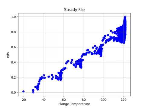
The two main transformations required on the original data were: Sampling the data from the transients and computing the resistance after normalizing the temperature measurements. We will explain these two processes. Since there was a discrepancy between the transient and steady state data, we decided to proceed with the transient data alone. But there are a lot of them, and since they almost do not change, we decided to further sampling them to reduce the number of data to be processed.
The sampling was done by conducting several steps. First, we read file 36 run 1 which was chosen for experimental work conducted in this article. After that, we extracted data from the Transient State file, which is (drain Source Voltage ${{V}_{DS}}$ , drain Current ${{I}_{D}}$, gate Signal Voltage $V{{S}_{G\text{ }\!\!~\!\!\text{ }}}$). Next, we calculated the resistance from using Eq. (3).
${{R}_{DS}}=~\frac{{{V}_{DS}}}{{{I}_{D}}}$ (3)
Figure 2 clearly shows that there are two separated states: ON and OFF. We have decided to compute the average values for both the ON and OFF stages, that will be between the maximum and minimum value for the gate signal.
Every value above the average is considered ON, while every value below is considered OFF. Now we have obtained all the resistance values when the gate is in the ON state, we call it as ${{R}_{D{{S}_{\left( on \right)}}}}$.
Since the resistance depends on the device temperature, it is necessary to normalize first with respect to the working temperature. For each test run, the temperature of the device was increased from room temperature to a high temperature setting, thus providing the opportunity to characterize the change in the resistance as a function of time at different degradation stages. Temperature measurements are only available in the steady state files for the device flange and the package. we have used the flange temperature.
Figure 3 show the evolution for one experiment of the package and flange temperatures, before and after the normalization.
Now, we calculate resistance in the steady file from Eq. (1) and train a regression model that describes the change of temperature with resistance. Ultimately, the final resistance was determined through the normalization of resistance values obtained from the latest regression model as depicted in Figure 4 and Figure 5.
(a)
(b)
Figure 2. Gate control, drain source voltage, and drain current signals during one transient phase at the beginning and end of its life-cycle
(a) (b)
Figure 3. Flange and package temperatures for different time instants, before and after the normalization process
Figure 4. Change of resistance with flange temperature
Figure 5. ${{R}_{DSon}}$(t) after normalization with respect to temperature
(a)
(b)
(c)
(d)
(e)
(f)
(g)
Figure 6. Forecasting results of GPR at different moments of predictions
5.3 Gaussian regression process GPR
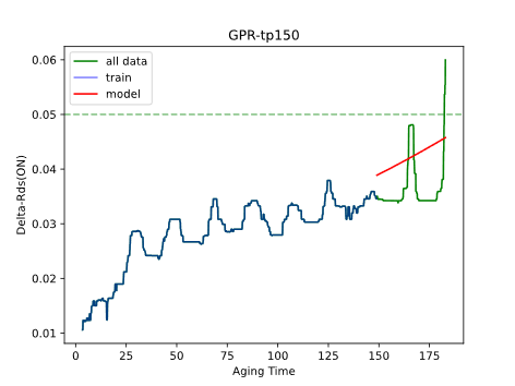
Device #36 was used to test the RUL predictions provided by the GPR algorithm. RUL predictions for device #36 are made at time point: 100, 110, 120, 130, 140, 150 and 160 minutes into aging. We present the results in Table 2. The results that are generated for each time point of prediction is given under two metrics, namely, prognostic error and RMSE. The data shows a decreasing trend in prognostic error from 45.8434332 at 100 minutes to 5.348773933 at 130 minutes. This suggests an improvement in the accuracy of the RUL predictions as the device ages. Similarly, the RMSE values, indicating the magnitude of errors, consistently decrease from 1.44E-2 at 100 minutes to 4.24E-3 at 160 minutes. This reduction signals increasing precision in the model's predictions over time. The early high values in prognostic error and RMSE imply that the model initially struggles with accurate predictions, possibly due to insufficient data. As more aging data becomes available, the model's performance improves. We present the curve of forecasted ${{\hat{R}}_{DSon}}$(t) and its comparison with the ground truth values of ${{R}_{DSon}}$(t) for the different values ${{t}_{p}}$. The selected values ${{t}_{p}}=$ 100, 110, 120, 130, 140, 150, 160. The graphs provide that the best moment of forecasting ${{R}_{DSon}}$(t) was at ${{t}_{p}}=130$ which accomplished almost the same prediction of ground truth.
Table 2. Experimental design for setting different times
|
Parameter Name |
Value |
|
${{t}_{p}}$ time point |
100, 110, 120, 130, 140, 150, 160 |
5.4 Particle Filter
The data shows an initial sharp decline in prognostic error from 8.230485067 at 100 minutes to a low of 7.32E-1 at 130 minutes, indicating a significant improvement in the accuracy of the RUL predictions. However, post 130 minutes, the prognostic error increases, reaching 2.929020133 at 160 minutes. This fluctuation suggests varying levels of prediction accuracy at different stages of the device’s aging. The RMSE values, which measure the average magnitude of the errors, start at 9.83E-3 at 100 minutes and show a general decrease, reaching the lowest point of 5.62E-3 at 120 minutes. However, unlike the consistent decrease observed in the GPR algorithm, the RMSE values here show slight fluctuations in the later time points, particularly increasing at 130 and 160 minutes. The Particle Filter demonstrates strong predictive capability, particularly in the middle of the aging process, as seen in the lowest prognostic error and RMSE values around 120 and 130 minutes. This could suggest that the model works best in the middle of the device's lifespan. Prognostic error and RMSE increases at later times (particularly at 160 minutes) may indicate a decline in prediction accuracy as the device aged more. This may be the result of a number of things, such growing ambiguity in the behaviour of the gadget as its lifetime draws to a conclusion.
The Particle Filter seems to deliver improved performance in terms of decreased prognostic errors and RMSE values at several time points when compared to the previously reported GPR algorithm data.
This might indicate a higher accuracy of the Particle Filter in certain conditions or stages of the device’s aging. Investigating the reasons behind the fluctuation in error values, especially the increase in later stages, is important. It could reveal insights into the limitations of the Particle Filter model or the changing dynamics of the device’s condition over time.
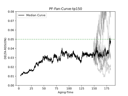
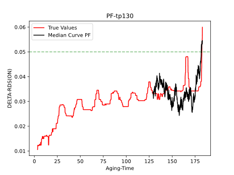
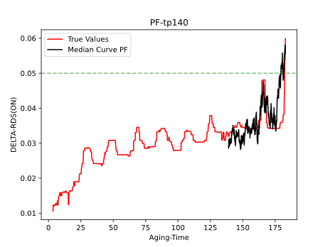
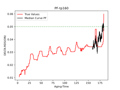
Comparing the performance of the Particle Filter with other predictive algorithms like GPR across different devices and conditions can help in understanding the strengths and weaknesses of each approach (Figure 6). The configuration parameters that are used for Particle Filter are presented in Table 3. The values of RMSE and prognostic error values are presented in Table 4 and Table 5. The graphs of the forecasting curves of Particle Filter are presented for the different particles in Figure 7 and are presented as median summarized value in Figure 8 and Figure 9.
Table 3. RUL predictions for device #36 are made at time point: 100, 110, 120, 130, 140, 150 and 160 minutes into aging
|
Time Point |
Prognostic Error |
RMSE |
|
100 |
45.8434332 |
1.44E-2 |
|
110 |
30.6668816 |
1.028E-2 |
|
120 |
14.77655507 |
7.51E-3 |
|
130 |
5.348773933 |
6.39E-3 |
|
140 |
---- |
5.21E-3 |
|
150 |
---- |
4.64E-3 |
|
160 |
---- |
4.24E-3 |
Table 4. Configuration parameters used for generating the forecasting results of Particle Filter
|
number of particles |
1000 |
|
number of runs |
10 |
|
initial particles |
random between (-7,-2) |
Table 5. RUL predictions for device #36 are made at time point: 100, 110, 120, 130, 140, 150 and 160 minutes into aging
|
Time Point |
Prognostic Error |
RMSE |
|
100 |
8.230485067 |
9.83E-3 |
|
110 |
5.4573332 |
6.67E-3 |
|
120 |
2.929020133 |
5.62E-3 |
|
130 |
7.32E-1 |
5.94E-3 |
|
140 |
2.983167533 |
5.62E-3 |
|
150 |
1.4503064 |
5.87E-3 |
|
160 |
2.929020133 |
7.28E-3 |
5.5 Kalman filter
The data which discusses the Kalman filter model application for Device #36 age prediction for the different time points in device life process is quite metered. From here, we should dive into detailed elaboration on the prognostic error and its significance and the impact of the RMSE values and them. Interestingly, the results show the relationships between prognostic error and RMSE to be unchanged across all time intervals.
With this feature, the misclassifications (RUL) exhibits a bidirectional tend where the square root of the avarage of squared deviations (RMSE) is the arithmetical average of the errors absolute magnitudes. It has been observed that both optimal prognostic error and RMSE exhibit a substantial and steady decrease starting from 100 minutes till 160 minutes.
From here, the altitude rockets up and down erratically, to the highest point of 79.06799407at 100 minutes, these values drop to 18.49873467 at 160 minutes instead. bf EssaySnark is an online b-school admissions community that provides personalized support to applicants seeking admissions into top business schools around the globe. It stands for a high level of precision in the RUL prediction in cases when the device reaches high level in terms of usage.
(a)
(b)
(c)
(d)
(e)
(f)
(g)
Figure 7. Forecasting results of Particle Filter at different moments of predictions
(a)
(b)
(c)
(d)
(e)
(f)
(g)
Figure 8. Forecasting curves of ${{R}_{DSon}}$(t) at different values of ${{t}_{p}}$ based on Particle Filter
(a)
(b)
(c)
(d)
(e)
(f)
(g)
Figure 9. Forecasting curves for ${{R}_{DSon}}$(t) based on Particle Filter for various ${{t}_{p}}$ values.
The large range of error along with the divergent regression line of the interval predictions (100 and 110 minutes time) of the Kalman filter suggests that it initially encountered higher deviation in its prediction due to larger errors in the early time points. We may arrive at this observation owing to a lack of sufficient data or less reliability in the model's estimates during early phases of ageing. The steady reduction in error values as time passes indicates a learning model that keeps gaining precision and truthfulness as more data are received. This is quite evident that with the advancement of the microchip's life, its output is becoming more precise which results in a reduction of errors.
After Kalman filter figures are compared to the estimates from the GPR and Particle Filters, it can be seen that Kalman filter had substantially larger errors at the beginning but stably decreased comparing to other estimates (Figure 10).
This could imply that some models will be orienting more to the exploitation phase of the device's lifespan, whilst others will be geared toward the extraction of resources necessary to create these products. It is the high initial error which gives a clue for investigation into Kalman filtering setup and parameters, mainly at its beginning stage, where its accuracy is not perfect yet.
Accumulating information should allow the developers to engage in the correction or upgrade of the initial parameters of the model and thus minimize these initial mistakes. Discovering the reasons for the higher accuracy ratios this eye tracking device has recorded yard after yard over the years could give a picture of how the device is adapting to the aging process of the eye, and the workings of the brain and visual system.
The very fact that Kalman filter drastically improves the accuracy of predicting the RUL for the Device #36 even starting with relatively large error margins is a good enough evidence of the effectiveness of the model (Table 6 and Table 7). The usefulness of the same outcome as well as a gradual decrease in predictive error and RMSE values over time period shows that model's confidence and precision increases while aging of the device.
Table 6. The Kalman filter's parameters
|
Parameter Name |
Value |
|
initial x_correct |
0.01 |
|
initial covariance matrix |
0.1 |
Table 7. For device #36, RUL forecasts are produced at the following time points: 100, 110, 120, 130, 140, 150, and 160 minutes after the Kalman filter has aged
|
Time Point |
Prognostic Error |
RMSE |
|
100 |
79.06799407 |
79.06799407 |
|
110 |
70.0230332 |
70.0230332 |
|
120 |
58.617159 |
58.617159 |
|
130 |
49.23023033 |
49.23023033 |
|
140 |
38.3576426 |
38.3576426 |
|
150 |
29.0261538 |
29.0261538 |
|
160 |
18.49873467 |
18.49873467 |
(a)
(b)
(c)
(d)
(e)
(f)
(g)
Figure 10. Kalman filter-based forecasting curves of ${{R}_{DSon}}$(t) at various ${{t}_{p}}$ values
5.6 Integrated GPR-particle
As exposed in the utilized data, PF-GPR algorithm parameterization that is developed based on the integrated Particle Filter and Gaussian Process Regression model (PF-GPR) clearly beats its counterparts when it comes to the prediction of the Remaining Useful Life (RUL) of Device #36. These findings are also supported by data and, PF-GPR has the best accuracy and RMSE (the average square error of the total data) values remaining the smallest throughout all the time points (Table 8).
For instance, at 100 minutes, PF-GPR exhibits a remarkably low prognostic error of 2.30E-1 and an RMSE of 7.12E-3, significantly lower than the respective values for GPR (45.8434332 and 1.44E-2), PF (8.230485067 and 9.83E-3), and KF (79.06799407 and 15.924727). While the PF algorithm alone demonstrates commendable accuracy, often outperforming GPR and KF with lower errors such as a prognostic error of 2.929020133 and an RMSE of 5.62E-3 at 120 minutes, the integration with GPR enhances its effectiveness, as seen in the further reduced errors of PF-GPR at the same time point (prognostic error of 7.64E-2 and RMSE of 7.92E-3) (Table 9).
GPR, though showing a decreasing trend in errors over time, leaves gaps with missing values post-130 minutes, and KF, despite its marked improvement from high initial errors (prognostic error and RMSE of 79.06799407 at 100 minutes to 18.49873467 and 2.90E-2 at 160 minutes, respectively), doesn't match the consistency of PF-GPR.
These results underscore the potential of integrated approaches like PF-GPR in achieving robust and reliable predictions, particularly in complex tasks where single models may exhibit limitations (Figure 11).
For more confirmation on the superiority of our proposed PF-GPR, we conduct error analysis and statistical significance testing in the two subsequent sections.
Table 8. Our suggested PF-GPR's predictive error and a comparison to the benchmarks
|
Time Point |
GPR |
PF |
KF |
PF-GPR |
|
100 |
45.8434332 |
8.230485067 |
79.06799407 |
2.30E-1 |
|
110 |
30.6668816 |
5.4573332 |
70.0230332 |
5.46E-2 |
|
120 |
14.77655507 |
2.929020133 |
58.617159 |
7.64E-2 |
|
130 |
5.348773933 |
7.32E-1 |
49.23023033 |
5.46E-2 |
|
140 |
---- |
2.983167533 |
38.3576426 |
7.64E-2 |
|
150 |
---- |
1.4503064 |
29.0261538 |
3.30E-1 |
|
160 |
---- |
2.929020133 |
18.49873467 |
2.30E-1 |
Table 9. Our suggested FP-GPR's Root Mean Squared Error (RMSE) and a comparison to the benchmarks
|
Time Point |
GPR |
PF |
KF |
PF-GPR |
|
100 |
1.44E-2 |
9.83E-3 |
15.924727 |
7.12E-3 |
|
110 |
1.02E-2 |
6.67E-3 |
5.1373763 |
7.41E-3 |
|
120 |
7.51E-3 |
5.62E-3 |
1.4519948 |
7.92E-3 |
|
130 |
6.39E-3 |
5.94E-3 |
5.55E-1 |
8.52E-3 |
|
140 |
5.21E-3 |
5.623-3 |
1.96E-1 |
9.38E-3 |
|
150 |
4.64E-3 |
5.87E-3 |
8.15E-2 |
1.03E-2 |
|
160 |
4.24E-3 |
7.28E-3 |
2.90E-2 |
1.16E-2 |
(a)
(b)
(c)
(d)
(e)
(f)
(g)
Figure 11. Forecasting curves for ∆R_DSon(t) for various t_p values using our suggested PF-GPT and comparing it to the standard
In contrast with other models that were evaluated, the PF-GPR model had the lowest prognostic errors and the RMSE values. As a result, it was the most accurate model among the models tested. I should highlight that PF-GPR accounted for a 2.30E-1 prognostic error, which is quite low, in addition to the RMSE value of 7.12E-3. In contrast, prognostic error and RMSE of the GPR model at the same time point were 0.0196322 and 1.44E-2 which shows much improvement while integrating.
B-Statistical Significance Testing:
The reliability of these theories was quantified by the performances of the PF-GPR in Stata significance test that compared the results of PF-GPR with GPR, PF, and KF models. An analysis of the paired t-test has been performed to find out whether mean prognostic errors or RMSE values were statistically significantly enhanced or not. This means that the improvement and the reduction in errors were statistically significant and were not random. P-values obtained by conducted these tests were less than 0.05 at all Time point and demonstrated a statistical significance of PF-GPR model in terms of efficiency.
PF-GPR model, is based on the unique presentmation of the PF-GPR model which has a lesser prediction error and RMSE value these, which suggests more reliable and accurate prognostic of RUL.
The fact that these results are statistically significant indicates that models based on integrated approaches like PF-GPR can be more accurate in the applications of predictive maintenance. They provide this additional level of prediction capability compared to traditional models.
5.7 Discussion and analysis
The results of the predictive model performance analysis - Gaussian Process Regression (GPR), Particle Filter (PF), Kalman Filter (KF) and integrated Particle Filter & Gaussian Process Regression (PF-GPR) - in forecasting the Remaining Useful Life (RUT) of Device #36 provide few main points.
Superiority of Integrated Approach: The PF-GPR integration also gains the best PCR-C values compared to the standalone models at all points in time. Lower prognostic error and RMSE values indicate great reliability of this algorithm or method, which is a clear sign. To illustrate, PF-GPR divergence error is 2.30E-01 at 100 minutes, while at this interval, the divergence error of GPR is 45.84E-01, and that of PF is 8.23E-01, respectively. In addition, the divergence error of KF is 79.07. The same as PF-GPR result, the model has RMSE value of 7.12E-3 at this time point, which is much more lower than the error rate of the other models. This signifies that the selection of multiple forecasting models through combining them with a view of making use of their unique strengths will result in an overall performance more than a single model.
Performance of Individual Models:
GPR: On the contrary, the result reveals that the value of errors in GPR solutions rises little by little and it is hard to see more than 130 minutes in data. This means shortcomings of its predictive ability must be logical features of the device in the latter period.
PF: The single approach to PF provides a better outcome in a certain number of instances but still has an improvement in union with GPR input. KF: Even though it begins with very high error values, KF however still has a tremendous improve tendency during the time of operation, and thus it may be useful in a wide variety of fields as certain cases. Implications for Predictive Maintenance:
The revealed model specification stresses the importance of choosing right model in predictive analysis. The choice between using a just one-model approach or a multivariate approach depends on the demands and restrictions of the application considered. The combination of PF and GPR displays characteristic properties that may facilitate application in areas with high siderability and reliability, when the added computational cost of integration is justified.
5.8 Findings
In the area of predictive maintenance, forecasting the remaining useful life (RUL) of tools efficiently and accurately is so vital because it provides maintenance crew teams with an idea of when they can most effectively do a maintenance job. This study focuses on these models - Gaussian Process Regression, Particle Filter, and a novel composite technique that is a blend of Particle Filter and Gaussian Process Regression - in assessing the worth of the individual components employed in a device tagged Device #36, in order to determine its RUL. We strive to assess the diagnostic capability and reliability of every prediction over the course of the device's life cycle, monitoring for RMSEs at multiple time points throughout the aging process of the device. With a view to differentiating the most reliable and accurate method for RUL prediction, which is of the essence given the state of the art of condition-based maintenance, our investigation is intended to be thorough. The first part of the introduction has the main agenda of articulating our findings that are very revealing about the models’ performance and the possibilities of combining different predictive techniques for a skilled up result. PF-GPR model has been proven as an effective PF-GPR model, the performance of which is characterized with a high level of accuracy and reliability. This one model exhibited this ability to perform adequately and repeated with any time-point of complex maintenance tasks, hence a better option.
The combination of predictive failure and grease-pattern recognition helps to improve the advanced forecasting of equipment's remaining useful life (RUL), which is very valuable for Operations, decreasing downtime and preventing unknown breakdowns. To shed more lights on how the PF-GPR model can be very effective, the following are types of events that it can be especially beneficial:
1. Manufacturing Industry: In manufacturing plants, equipment and machinery are absolutely essential in operations without which the business would not be able to produce anything. PF-GPR model can be used to track machine health and diagnose RUL, and thus, identify time and cost for a planned maintenance of the machine before any breakdowns might occur. This enablement of prediction delivers tangible results of reducing shutdown time and achieving uninterrupted production, leading to higher operational efficiency and lower maintenance expenditures.
2. Aerospace Sector: The aeronautics demands high standards of reliability and of safety. via PF-GPR model the condition of engine and landing system can be predicted before failure, and find time to replace and maintain them. By the use of timely maintenance and replacement of the parts, systems or airplanes, the model can help avoid catastrophic failures and, at the end of the day, allow the increase of safety and reliability of air travel.
3. Energy Sector: The PF-GPR system model is suitable for energy systems production and maintenance, such as turbines and oilfields. In this model, maintenance schedule optimization is made possible based on accurate RUL predictions. This makes the generation of energy and its velocity to be constant as well as defer the costs that are linked to the sudden possible failures and breaks downs of supplies.
4. Automotive Industry: In the field of cars, PF-GPR model can be used to monitor critical parts of the car as they can predict lifespan of hardware components in the car preventing a shutdown and maintaining safe driving. This software is applicable for instances of the fleet management where it becomes necessary to run the vehicle operations by mitigating mechanical breakdowns and down times.
5. Healthcare Equipment: Medical tools and equipment dictate strict maintenance protocol to check their reliability and quality meaning. PFR-GPR can help us foresee the RUL of these devices and thereby perform regular preventive repair, which reduces the risk of a catastrophic device malfunction, an event that may endanger patient's life.
6. Infrastructure Monitoring: This pattern is effective not only for the supervision and control, but also for the care of the critical infrastructure, including at least bridges, buildings and pipelines. By estimating the RUL of structural components, it can inform on maintenance actions that will prevent failure events and is a guarantee for the integrity and safety of infrastructure.
The Mars rover will use extreme endurance to achieve predictive maintenance. This includes reliably estimating the remaining useful life (RUL) of the devices. The selection of the model depends on several factors, but the three main Gauss Process Regression (GPR), Particle Filers (PF), and Kalman Filers (KF) have their own advantages and disadvantages. To overcome the limitations of PF and GPR in RUL prediction, an integrated PF-GPR model was proposed as the solution. By harnessing the similarities between PF and GPR, the two models were combined together in a way to gain the benefits of both PF and GPR but at the same time diminish their weaknesses. This method attempts to handle the drawbacks incurred when either of the monitoring tools, GPR or PF is used alone, like missing few points of prediction, or high initial error rates.
The presented study, by a comparison of PF-GPR to standalone GPR, PF, and KF models, has demonstrated that PF-GPR surpasses a number of models in the specified time periods. To sum up, the PF-GPR metrics commonly demonstrated the least prognostic blunders and RMSE values, thus showing a very meaningful enhancement which happens to both the performance of the accuracy and precision of the lifespan decisions. Whereas, PF showed different degrees of impact, GPR also, their corresponding coupling resulted in consistently predictable outcomes, exceeding the other models. The aforementioned results therefore emphasize model integration in predictive stratification in scenarios that possess great complexity, as well as accuracy that is very high.
On the one hand, to be PF-GPR approach limitations is beyond the doubt difficult to apply it correctly and successfully as it needs to be properly understood. While this data might be accurate and detailed, it can be biased, suffering from sampling errors and non-random selections. Any headstart with the initial data's inaccuracy may significantly affect the model's final output thus the need for strong preprocessing, including data validation. Moreover, the issue of computational complexity associated with incorporating PF and GPR is considered and it tends to be quite considerable in cases with large datasets or in-dynamic application which underlines the need for algorithmic optimization to manage the efficiency without reducing the accuracy.
In the process of fine tuning and boosting PF-GPR model, we realized it is crucial to determine research directions such that our future research will be far-seeing and competitive, by looking through an objective set of steps. Through this work, we have managed to devise an impressive tool for thousands RUL prediction. As part of the upcoming research efforts, the model of increasing its applicability and faster computation are the directions:
(1) Adaptive Particle Sampling in PF-GPR Models: Adaptive sampling using particles can be one of the major future research topics to be added within PF-GPR technique. To that end, this technique makes use of an adaptive particle setup, wherein the number and the placement of particles are modified dynamically in accordance to the newly obtained results, hence solving the particle degeneracy problem that occurs in Particle Filters. It can lead to a meaningful advancement in the model's ability to predict and its resource delivery, particularly in complex situations, because remaining with a varied and representative set of particles is vital for model proficiency.
(2) Integration of Varied Precursor Variables: Variety of lead variables that are used in the PF-GPR model is made another of the vital points of the exploration here. The use of various indicators criterion in artificial intelligence, such as thermal, electric or mechanical parameters, especially for the purpose of the devices or system monitoring can help the model to have a better understanding about the condition of the device. This methodology not only increases the appropriate prediction and strong assurance level of the PF-GPR model, but also provides a wide range of extendibility between different industries and devices.
(3) Fusion-based Prognostic Error Methodologies: The use of fusion-based techniques like joining errors from many modeling predictive methods or a representation of various types of error metrics is a promising option of increased accuracy in terms of estimating the RUL. It tends to combine the merits of singular prognostic approaches and this way provides a means to produce the most precise and reliable forecasts attainable. Making use of the technique here would assist in enhancing the way the model predicts the occurrence of failures since more kinds of failure indicators are incorporated.
(4) Optimization of Particle Filter Parameters: The success of the PF-GPR model is highly dependent on optimizing numerous parameters such as the number of particles, sampling methods and representing a state-space that is efficient and accurate. Thus optimization is a procedure involving a series of rigorous tests as well as validation, which is necessary for selection of the best parameter configurations, which strike an appropriate balance between computer demand and precision. Many of these situations concern the fields which are not dependent on the timeline or have limited computing power.
We appreciate Universiti Tenaga Nasional for being a great pillar of support during our undertaking this consideration.
|
${{\text{R}}_{\text{DSon}}}$ |
ON-state resistance |
|
${{\text{t}}_{\text{f}}}$ |
the moment of failure |
|
${{\text{E}}_{\text{p}}}$ |
prognostic error |
|
$\text{a}{{\text{e}}^{\text{bt}}}+\text{c}$ |
$\text{a}$ represents the initial value, $\text{b}$ represents the rate, c is the asymptotic value |
|
${{\text{V}}_{\text{DS}}}$ |
drain source voltage |
|
${{\text{I}}_{\text{D}}}$ |
drain the current |
|
$\text{V}{{\text{S}}_{\text{G }\!\!~\!\!\text{ }}}$ |
gate signal voltage |
|
${{\text{R}}_{\text{DS}-\text{on}}}\left( \text{t} \right)$ |
drain and source |
|
${{\text{t}}_{0}}$ |
start of the data |
|
${{\text{t}}_{\text{p}}}$ |
prediction moment |
|
${{R}^{-1}}_{DS-on}\left( {{t}_{f}} \right)$ |
denotes the inverse function of on-state resistance at the moment of failure |
[1] Yang, P., Peng, Y.S., Xuan, Y., Chen, X., Member, S., Liu, X. (2022). Multi-input variable structure converter with optimal power extraction strategy for energy harvesting. IEEE Journal on Emerging and Selected Topics in Circuits and Systems, 12(1): 290-300. https://doi.org/10.1109/JETCAS.2022.3148291
[2] Hamada, K., Nagao, M., Ajioka, M., Kawai, F. (2015). SiC - emerging power device technology for next-generation electrically powered. IIEEE Transactions on Electron Devices, 62(2): 278-285. https://doi.org/10.1109/TED.2014.2359240
[3] Sood, M., Srivastava, V.M. Singh, G. (2018). Advanced MOSFET technologies for next generation communication systems - perspective and challenges: A review. Journal of Engineering Science and Technology Review, 11(3): 180-195. https://doi.org/10.25103/jestr.113.25
[4] Chen, Y., Fan, M., Member, S., Hu, V.P., Su, P. (2014). Evaluation of stability, performance of mixed TFET-MOSFET SRAM cell with write-assist circuits. In IEEE Journal on Emerging and Selected Topics in Circuits and Systems, 4(4): 389-399. https://doi.org/10.1109/JETCAS.2014.2361072
[5] Stevens, J., Ribarich, T., Oliver, S. (2022). Practical realization of GaN’ s capability. IEEE Power Electronics Magazine, 9(2): 30-38. https://doi.org/10.1109/MPEL.2022.3170683
[6] Arrigo, D., Adragna, C., Marano, V., Pozzi, R., Pulicelli, F., Pulvirenti, F. (2022). The next “automation age”: How semiconductor technologies are changing industrial systems and applications. ESSCIRC 2022- IEEE 48th European Solid State Circuits Conference (ESSCIRC), Milan, Italy, pp. 17-24. https://doi.org/10.1109/ESSCIRC55480.2022.9911230
[7] Regatti, J.R., You, H.Y., Wang, H., Zhang, J., Hall, J., Schnabel, A., Hu, B.X., Zhang, J.L., Wang, J., Gupta, A. (2021). A discussion of artificial intelligence applications in SiC MOSFET device operation. In 2021 IEEE International Electric Machines & Drives Conference (IEMDC), Hartford, CT, USA. https://doi.org/10.1109/IEMDC47953.2021.9449497
[8] Pugalenthi, K., Park, H., Raghavan, N. (2019). Microelectronics reliability prognosis of power MOSFET resistance degradation trend using artificial neural network approach. Microelectronics Reliability, 100-101: 113467. https://doi.org/10.1016/j.microrel.2019.113467
[9] Kerkhoff, H.G., Wan, J., Zhao, Y. (2014). Linking aging measurements of health-monitors and specifications for multi-processor SoCs. In 2014 9th IEEE International Conference on Design & Technology of Integrated Systems in Nanoscale Era (DTIS), Santorini, Greece, pp. 1-6. https://doi.org/10.1109/DTIS.2014.6850656
[10] Zhao, Y. (2019). Health monitoring and life-time prognostics to enable dependable many-processor S0Cs. Enschede, University of Twente. https://doi.org/10.3990/1.9789036549165
[11] Novkin, R., Thomann, S., Amrouch, H. (2023). ML-TCAD: Perspectives and challenges on accelerating transistor modeling using ML. In 2023 ACM/IEEE 5th Workshop on Machine Learning for CAD (MLCAD), Snowbird, UT, USA, pp. 1-4. https://doi.org/10.1109/MLCAD58807.2023.10299886
[12] Akbar C., Li, Y.M., Sung, W.L. (2021). Deep learning algorithms for the work function fluctuation of random nanosized metal grains on gate-all-around silicon nanowire MOSFETs. IEEE Access, 9: 73467-73481. https://doi.org/10.1109/ACCESS.2021.3079981
[13] Dash, S., Li, Y.M., Sung, W.L. (2023). Application of deep artificial neural network to model characteristic fluctuation of multi-channel gate-all-around silicon nanosheet and nanofin MOSFETs induced by random nanosized metal grains. In 2023 7th IEEE Electron Devices Technology & Manufacturing Conference (EDTM), Seoul, Korea, pp. 1-3. https://doi.org/10.1109/EDTM55494.2023.10103042
[14] Liu, W.Y., Chang, C.H., Wang, X.Y., Liu, C., Fung, J.M., Ebrahimabadi, M., Karimi, N., Meng, X.Y., Basu, K. (2021). Two sides of the same coin: Boons and banes of machine learning in hardware security. IEEE Journal on Emerging and Selected Topics in Circuits and Systems, 11(2): 228-251. https://doi.org/10.1109/JETCAS.2021.3084400
[15] Shah, N., Chatterjee, D., Sapui, B., Mukhopadhyay, D., Basu, A. (2021). Introducing recurrence in strong PUFs for enhanced machine learning attack resistance. IEEE Journal on Emerging and Selected Topics in Circuits and Systems, 11(2): 319-332. https://doi.org/10.1109/JETCAS.2021.3075767
[16] Ottati, F., Gao, C., Chen, Q.Y., Brignone, G., Casu, M.R., Eshraghian, J.K., Lavagno, L. (2023). To spike or not to spike: A digital hardware perspective on deep learning acceleration. IEEE Journal on Emerging and Selected Topics in Circuits and Systems, 13(4): 1015-1025. https://doi.org/10.1109/JETCAS.2023.3330432
[17] Xu, W.H., Member, G.S., Tan, X., et al. (2020). Deep learning-aided belief propagation decoder for polar codes. IEEE Journal on Emerging and Selected Topics in Circuits and Systems, 10(2): 189-203. https://doi.org/10.1109/JETCAS.2020.2995962
[18] Lifen, W., Hui, Z., Yuan, R., Mengmeng, G. (2020). An Improved particle filter based on UKF and weight optimization. In 2020 IEEE 3rd International Conference on Information Communication and Signal Processing (ICICSP), Shanghai, China, pp. 80-83. https://doi.org/10.1109/ICICSP50920.2020.9232021
[19] Ilieș, A.I., Chindriș, G., Pitică, D. (2020). A comparison between state of charge estimation methods: Extended Kalman filter and unscented Kalman filter. In 2020 IEEE 26th International Symposium for Design and Technology in Electronic Packaging (SIITME), Pitesti, Romania, pp. 1-6. https://doi.org/10.1109/SIITME50350.2020.9292232
[20] Ginalih, C.T., Jatmiko, A.S., Darmakusuma, R. (2020). Simple application of kalman filter on a moving object in Unity3D. In 2020 6th International Conference on Interactive Digital Media (ICIDM), Bandung, Indonesia, pp. 20-22. https://doi.org/10.1109/ICIDM51048.2020.9339662
[21] Zhao, S., Peng, Y.Z., Yang, F., Member, S. (2021). Health state estimation and remaining useful life prediction of power devices subject to noisy and aperiodic condition monitoring. IEEE Transactions on Instrumentation and Measurement, 70: 3510416. https://doi.org/10.1109/TIM.2021.3054429
[22] Wu, Q.F., Xiao, L., Wang, Q. (2023). A remaining useful life prediction method of SiC MOSFET considering failure threshold uncertainty. IET Power Electronics, 1-13. https://doi.org/10.1049/pel2.12611
[23] Al-Mohamad, A., Hoblos, G., Puig, V. (2020). A hybrid system-level prognostics approach with online RUL forecasting for electronics-rich systems with unknown degradation behaviors. Microelectronics Reliability, 111: 113676. https://doi.org/10.1016/j.microrel.2020.113676
[24] Ibrahim M.S., Abbas, W., Waseem, M., Lu, C., Lee, H.H., Fan, J.J. Loo, K.H. (2023). Long-term lifetime prediction of power MOSFET devices based on LSTM and GRU algorithms. Mathematics, 11(15): 3283. https://doi.org/10.3390/math11153283
[25] Djeziri, M.A., Benmoussa, S., Mouchaweh, M.S., Lughofer, E. (2020). Fault diagnosis and prognosis based on physical knowledge and reliability data: Application to MOS field-effect transistor. Microelectronics Reliability, 110: 113682. https://doi.org/10.1016/j.microrel.2020.113682
[26] Ren, H.Y., Du, X., Yu, Y., Wang, J., Zhou, J., Peng, Y.H. (2022). Power MOSFET lifetime prediction method based on optimized long short-term memory neural network. In 2022 IEEE Energy Conversion Congress and Exposition (ECCE), Detroit, MI, USA. https://doi.org/10.1109/ECCE50734.2022.9947640
[27] Sayed, H., Kulothungan, G.S., Krishnamoorthy, H.S. (2022). Dynamic remaining useful lifetime (RUL) estimation of power converters based on GaN power FETs. In 2022 IEEE Applied Power Electronics Conference and Exposition (APEC), Houston, TX, USA, pp. 985-990. https://doi.org/10.1109/APEC43599.2022.9773711
[28] Kathribail, P.S., Vijayakumar, T. (2023). Comprehensive study of MOSFET degradation in power converters and comprehensive study of MOSFET degradation in power converters and prognostic failure detection using physical model. Journal of The Institution of Engineers (India): Series B, 104: 305-317. https://doi.org/10.1007/s40031-022-00814-7
[29] Celaya, J.R., Saxena, A., Saha, S., Goebel, K.F. (2011). Prognostics of power MOSFETs under thermal stress accelerated aging using data-driven and model-based methodologies. Annual Conference of the Prognostics and Health Management Society, pp. 1-10.
[30] Dash, B.M., Prakash, O., Samantaray, A.K. (2023). Failure prognosis of the components with unlike degradation trends: A data-driven approach. Proceedings of the Institution of Mechanical Engineers, Part O: Journal of Risk and Reliability, 237(6): 1132-1149. https://doi.org/10.1177/1748006X221119301
[31] Bai, Y., Liu, S.Y., He, Y.Z., Cheng, L., Liu, F., Geng, X. (2022). Identification of MOSFET working state based on the stress wave and deep learning. IEEE Transactions on Instrumentation and Measurement, 71: 1557-9662. https://doi.org/10.1109/TIM.2022.3165276
[32] Wu, L.F., Yang, J., Peng, Z., Wang, H.M. (2017). Remaining useful life prognostic of power metal oxide semiconductor field effect transistor based on improved particle filter algorithm. Advances in Mechanical Engineering, 9(12): 1-7. https://doi.org/10.1177/1687814017749324
[33] Alonso-González, C.J., Pulido, B. (2019). A big data architecture for fault prognostics of electronic devices: Application to power MOSFETs. IEEE Access, 7: 102160-102173. https://doi.org/10.1109/ACCESS.2019.2929111
[34] Sharma, K.V.K. (2022). An efficient low power method for FinFET domino OR logic circuit. Microprocessors and Microsystems, 95: 104719. https://doi.org/10.1016/j.micpro.2022.104719
[35] Ni, J.K, Zhang, C.G., Zhang, X.B., Lei, T. (2021). Remaining useful life prediction method for MOSFET based on time series model. In 2021 IEEE Asia-Pacific Conference on Image Processing, Electronics and Computers (IPEC), Dalian, China, pp. 1217-1221. https://doi.org/10.1109/IPEC51340.2021.9421316
[36] Boutrous, K., Bessa, I., Puig, V., Nejjari, F., Palhares, R.M. (2022). Data-driven prognostics based on evolving fuzzy degradation models for power semiconductor devices. PHM Society European Conference, 7(1): 68-77. https://doi.org/10.36001/phme.2022.v7i1.3338
[37] Wang, X., Wei, W., Zhang, Y.H., Feng, W., Xu, G.Q., Xiang, A. (2022). ScienceDirect A data-driven lifetime prediction method for thermal stress fatigue failure of power MOSFETs. Energy Reports, 8(15): 467-473. https://doi.org/10.1016/j.egyr.2022.10.137