Assia Aouachria![]() | Moussa Anoune
| Moussa Anoune![]() | Soraya Tebbal
| Soraya Tebbal![]() | Zeroual Aouachria*
| Zeroual Aouachria*![]()
© 2023 IIETA. This article is published by IIETA and is licensed under the CC BY 4.0 license (http://creativecommons.org/licenses/by/4.0/).
OPEN ACCESS
In the endeavor to halt the transmission of infectious diseases, containment and isolation emerge as pivotal preventive strategies. The elucidation of disease spread dynamics, through the lens of mathematical models, is instrumental in forecasting epidemiological trajectories. This study presents an augmented Susceptible-Infected-Recovered (SIR) model, assimilating these preventive measures, to scrutinize the propagation of COVID-19 since its initial emergence. The combat against this pandemic has predominantly hinged upon non-pharmaceutical interventions (NPIs) including, but not limited to, mask utilization, physical distancing, patient isolation, contact quarantine, and hand hygiene. The focal point of our investigation lies in the examination of the influence of susceptible population containment and infected individual isolation on the evolution of the ongoing outbreak. The basic reproductive number, an indicator of contagiousness, is analyzed over the course of the outbreak, yielding promising outcomes.
Susceptible-Infected-Recovered (SIR) model, COVID-19, containment, isolation, Ain-Touta City, basic reproductive number
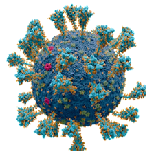
The global landscape has been dramatically altered by the emergence of a novel infectious disease, exhibiting profound impacts on human health, medical infrastructure, economies, and societal structures worldwide. The exigency for the implementation of host-based control measures, encompassing both non-pharmaceutical interventions (NPIs) and pharmaceutical interventions (PIs), to curtail the deleterious effects of this pandemic, is underscored by numerous studies [1, 2]. Illustratively, China's proactive and comprehensive response to the early stages of the disease exemplifies the necessity of such interventions. The highly transmissible nature of the causative agent, the SARS-CoV-2 virus, which is primarily spread via droplets (Figure 1), necessitates stringent control measures. These include, but are not limited to, expansive testing, meticulous contact tracing, large-scale isolations, compulsory quarantines, travel restrictions, border closures, social distancing mandates, school closures, long-term detention orders, and comprehensive lockdowns. The burgeoning crisis of the Coronavirus Disease 2019 (COVID-19) has galvanized a unified response from the global community, as evidenced by the escalating numbers of confirmed cases and fatalities. A representative case study, detailing daily cases, recoveries, and deaths in Algeria is presented in Figure 2. Furthermore, Figure 3 offers a projected roadmap of hospital admissions within England, highlighting the potential strain on medical resources.
The elucidation of COVID-19 transmission dynamics necessitates the application of mathematical modeling, facilitating the swift prediction of disease propagation and an evaluation of the efficacy of diverse intervention strategies. In the realm of infectious disease modeling, the basic reproduction number (ℛ0) serves to quantify the initial growth rate of a disease within a fully susceptible population. It provides critical insight into the infectiousness and the propagation rate of the disease in the absence of any intervention. The estimation of ℛ0 is of paramount importance for public health officials and governmental bodies. It allows for informed planning and the execution of effective response strategies to mitigate the spread of the disease. The application of mathematical models in the context of infectious diseases constitutes a potent tool, instrumental in shaping management policies and forming an integral part of the current toolkit deployed against the COVID-19 pandemic [3]. The incorporation of social distancing analyses via mathematical models has proven effective in curtailing the spread of the COVID-19 infection [3-9].
In the face of an outbreak, the timely deployment of appropriate control measures, including NPIs and PIs, is critical. During such crises, a collaborative approach across diverse societal sectors, under the guidance of the government, is essential. Scientists and technology experts are urged to leverage all available resources to assist the government in its battle against the epidemic.
The basic reproduction number (ℛ0) for an infectious disease denotes the predicted number of new cases directly caused by an index case within a susceptible population. In response to COVID-19, mathematical models have been rapidly utilized to project future transmission and outbreak scenarios, alongside potential infection control strategies [10-15]. The aim of this study is to forecast future transmission and outbreak dynamics using effective mathematical modeling tools. In this analysis, projections are viewed as performative actors with life potential through their implementation assemblies [15, 16]. Drawing on the seminal work of Michel Callon and others in the field of economics, it is recognized that models are not merely passive observers, but actively shape and create realities, engendering performative effects [17, 18]. Models take into account their social relationships, implicitly incorporating them into their assumptions and calculations [19, 20].
The primary objective of this study is to forecast the ramifications of isolation and confinement measures on a practical scale, and to discern potential limitations in their enactment. These measures are encapsulated by the alpha and delta parameters within the model diagram, with the system of equations mirroring the dynamics of the disease.
Figure 1. A scientifically accurate atomic model of the SARS-CoV-2 virus, CC BY-SA 4.0 [1]
Figure 2. Daily cases, recoveries, and deaths in Algeria [2]
Figure 3. Roadmap 1 projections for the number of hospital admissions in England
In order to model diseases that persist over an extended period, it is crucial to account for the demographic effect of the population, considering births and deaths. The population is divided into three distinct classes for modelling purposes. The first class represents the susceptible population (S), which consists of individuals who are at risk of being infected. The second class represents the infected population (I), comprising individuals who have contracted the disease. In most cases, once a person is infected, they become immune and are unlikely to be infected again. Therefore, the infected individuals eventually transition to a class of recovery or remission. In this model, we assume that the number of deaths is minimal compared to the number of recoveries. Thus, individuals in the population are either susceptible (capable of getting the disease), infected (capable of infecting others), or recovered (immune and unable to catch or transmit the disease).
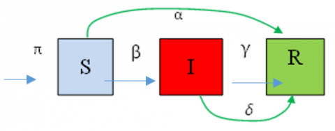
The SIR model is based on the assumption that the spread of an epidemic is influenced by the nature and frequency of contact between asymptomatic individuals and symptomatic infected individuals (Figure 4). These contacts occur through various social interactions, such as handshakes, hugs, close proximity (addressed by distancing measures), and professional relationships. To account for the impact of births within the susceptible population, the SIR model can be extended by introducing a birth rate parameter (π).
The objective of isolation measures is to separate infected individuals from uninfected ones to prevent the spread of the virus. The effectiveness of isolation is determined by the containment rates of susceptible individuals (α) and the isolation of infectious individuals (δ).
The proposed SIR model is an extension of the classic Kermack and McKendrick model [21, 22] and incorporates the effects of containment on the susceptible and infectious populations. The fraction of susceptible individuals who are likely confined is denoted as αS, while the fraction of uncontained susceptible individuals is (1-α).S. The fraction of uncontained infected individuals who are likely to infect others is represented by (1-δ).I, where δ is the infection rate. The fraction of infected individuals who are confined is δI. Additionally, the birth density of the susceptible population is denoted as π. The recovered population (R) includes individuals who have been removed from the infected population, represented by γ.I, where, γ is the recovery rate.
Figure 4. Schematic of the model of the system
Hence, the model can be formulated as a system of ordinary differential equations:
$\begin{gathered}\frac{d S}{d t}=\pi-\beta(1-\alpha)(1-\delta) S I-\alpha S \\ \frac{d I}{d t}=\beta(1-\alpha)(1-\delta) S I-\gamma I-\delta I \\ \frac{d R}{d t}=\alpha S+\gamma I+\delta I\end{gathered}$ (1)
Note that the system of equations includes the infected population (I), which represents the core aspect of the pandemic spread. To investigate the impact of the disease within a given time period, various initial conditions are considered for solving this system of differential equations.
Let us begin by considering the early stage of the disease, where the birth rate (π) is negligible, and there are no confinement or isolation measures in place (α=δ=0). Assuming the initial condition as:
$\mathrm{S}(\mathrm{t}=0)=\mathrm{S}_0=1$ (2)
Initially, there are no cures or deaths (γ=0). These assumptions imply that:
$\mathrm{S}+\mathrm{I}+\mathrm{R}=\mathrm{N}=$ Cte (3)
The coupled system of Eq. (1) takes the following form:
$\frac{d I}{d t}=\beta S_0 I$ (4)
The solution to this equation is given by the expression:
$I=I_0 e^{\beta S_0 t}$ (5)
with S0=1, at the beginning of the disease, the infection rate (β) can be expressed and calibrated based on the data from the initial period of infection as:
$\beta=\frac{\ln \frac{I^*}{I_0}}{t^*}$ (6)
For example, in the case of Ain-Touta (in Algeria) during the onset of the disease (March 1 to 7, 2020), based on the corresponding statistics, the value of the infection rate (β) was approximately 0.188. Thus, the epidemic tends to grow exponentially without any consideration for mortality or recovery. To measure the rate at which the infected population increases or decreases, we can use the concept of doubling time. The doubling time represents the time it takes for the population to double in size. It is a more comprehensible parameter compared to the exponential growth rate itself. The doubling time for the number of infected cases is expressed as:
$\tau^*=\frac{\ln (2)}{\beta S_0}=\frac{\ln (2)}{\beta}$ (7)
For β=0.188, the doubling time is approximately 3.687.
Now, let us consider the second phase of the epidemic, specifically the period from March 8 to March 19, 2020. We continue to assume a negligible birth rate (π=0) and no confinement or isolation measures have been implemented yet (α=δ=0). The system of Eq. (1) takes the following form:
$\left.\begin{array}{c}\frac{d S}{d t}=-\beta S I \\ \frac{d I}{d t}=\beta S I-\gamma I \\ \frac{d R}{d t}=\gamma I\end{array}\right\}$ (8)
This system has two characteristic stationary points. The first one is defined by:
$\frac{d S}{d t}=0$, which gives $(\mathrm{S}, \mathrm{I}, \mathrm{R}=(0,0,0)$ (9)
The second one is defined by:
$\frac{d I}{d t}=0$, which gives $(\mathrm{S}, \mathrm{I}, \mathrm{R})=(\gamma / \beta, 0,0)$ (10)
In this case, $\mathscr{R}_0=\beta / \gamma \quad$ and $\quad \frac{d I}{d t}$ is necessarily positive, indicating an increasing number of infections. Integrating the first two equations from 0 to ∞, we obtain:
$\log (S(\infty))=\Re_0(S(\infty)-1)$ (11)
Integrating between the start and the end of the second period, we obtain the transmission rate β:
$\beta=\frac{\ln \frac{S(19)}{S(8)}}{\int_8^{19} I(t) d t}=1.1$ (12)
Assuming that the average duration in the infected compartment (I) is approximately: $\frac{1}{\gamma} \approx 1$, we find that before isolation,
$\mathscr{R}_0=\frac{\beta}{\gamma}=1.1$ (13)
During this period, the disease spread slowly.
We consider the model (1) with confinement (α>0) and isolation (δ>0). Since the cure population, R, depends on the populations S and I, and the latter are independent of R, we can focus our study on the SI system. In the following analysis, we assume that π>0 to account for new births. The epidemic, for a certain period, can be described by the transformed system (1):
$\begin{aligned} & \frac{d S}{d t}=\pi-\beta(1-\alpha)(1-\delta) S I-\alpha S \\ & \frac{d I}{d t}=\beta(1-\alpha)(1-\delta) S I-\gamma I-\delta I\end{aligned}$ (14)
The stationary points of the system are obtained by solving this algebraic system when all S(t) and I(t) derivatives are equal to zero. We denote the equilibrium point without disease as E0 (S, I) and the equilibrium point with disease as E* (S*, I*). Cancelling the derivatives yields:
$E_0=\left(\frac{\pi}{\alpha}, 0\right)$ (15)
$E^*=\left(\frac{\gamma+\delta}{\beta(1-\alpha)(1-\delta)}, \frac{\pi-\alpha S^*}{(\gamma+\delta)}\right)$ (16)
We observe that the endemic equilibrium point is positive if (π-αS*) is positive, which requires the basic reproduction rate expression:
$\mathcal{R}_0=\frac{\beta(1-\alpha)(1-\delta)}{\gamma+\delta}>1$ (17)
It is important to note that the expression of ℛ0 depends on the specific cases being considered (isolation and confinement). Controlling the basic reproduction number ℛ0 to be less than 1 is crucial for ending an epidemic, such as COVID-19. By reducing contact, through containment and isolation measures (α, δ), these rates have gradually decreased from 3 per week to less than 1. By increasing the rate of confinement (α) for susceptible individuals and the rate of isolation (δ) for infected individuals, we can reduce ℛ0 and make it less than unity (ℛ0<1). This indicates a decrease in the number of infected individuals towards extinction. For instance, if we had 10,000 patients at the beginning of the epidemic, we would expect to have 30,000 the following week and 90,000 two weeks later. However, according to the $\mathcal{R}_0$ formula, if we increase the rates of containment for susceptible individuals and isolation for infected individuals (whether declared or not), we can make ℛ0<1, leading to a decrease in the number of infected individuals. Conversely, if ℛ0 remains greater than 1, the number of infected individuals will continue to increase each day, and the epidemic will persist over time since the endemic equilibrium point, in this case, is globally asymptotically stable. It is worth noting that this analysis of the basic reproduction number is closely linked to the study, as it is expressed based on the parameters of preventive measures such as isolation and confinement (α and δ).
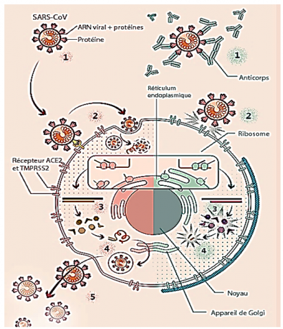
To properly interpret the results of mathematical modeling, it is crucial to understand the behavior of the virus within the environment where its life cycle takes place (see Figure 5).
Figure 5. Viral cycle of SARS-CoV-2 and therapeutic targets
The SARS-CoV-2 virus enters the body through the respiratory tract, specifically the nose and mouth. Its surface proteins interact with the ACE2 receptor present on the surface of cells that line our airways. Another cellular protein called TMPRSS2 facilitates the virus's entry into the host cell. Once inside, the virus hijacks the host's cellular machinery to replicate itself. Multiple copies of the virus are produced, which then go on to infect new cells. It is important to note that our study focuses on the dynamics of the disease caused by this virus in a broader societal context, rather than the specific dynamics of viral propagation within the human body. In general, the progression of each workforce aligns with the pace of the epidemic. Three curves, represented by different colours, are displayed side by side. The blue curve signifies the decreasing evolution of the population, indicating a reduction in numbers due to contamination. The green curve represents the evolution of the population of infected individuals over time, belonging to compartment I. However, this curve exhibits three distinct aspects: an ascending phase corresponding to the virulent stage of the epidemic, commonly known as "the peak" of the epidemic. The location and amplitude of this peak serve as relative indicators of the epidemic's strength and timing. The decline phase is linked to the progressive extinction of the epidemic.
6.1 Effects of initial boundary conditions
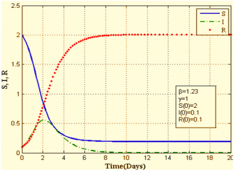
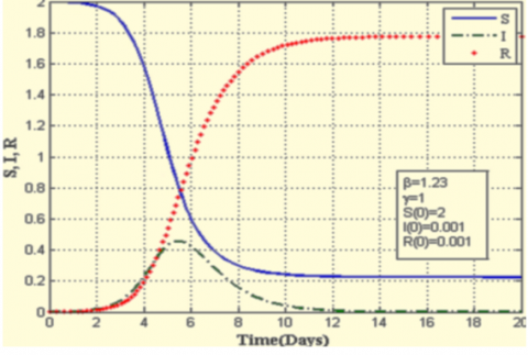
Figure 6 illustrated the COVID-19 transmission and dynamics as a function of the initial conditions. The contamination curve lacks symmetry, which means the phase of extinction can spread over time, unlike the initial stages of the epidemic. The tendency for the curve to flatten is a more realistic indicator of the epidemic's slowdown, Figure 6(a), 6(b) and 6(c), suggesting a reduction in the number of infected individuals, albeit with a longer period before the epidemic is completely extinguished. This flattening of the infection curve is strongly associated with the health protocol implemented during confinement.
(a)
(b)
(c)
Figure 6. COVID-19 transmission and dynamics as a function of the initial conditions for β=1.23 and γ=1
The curves in Figure 6 vividly illustrate the transmission behaviour and dynamics of the pandemic, influenced by the initial conditions of the coronavirus outbreak. These curves in Figure 6 are plotted for a contact rate (β) of 1.23 and a rate of recovery for infected individuals (γ) of 1. It can be observed that more severe conditions lead to an increase in the number of infected individuals, eventually reaching a peak. For instance, in Case 1 (Figure 6(a)), the proportion and number of infected individuals reach a maximum of 0.51 on the second day of the disease onset, which then drops to 0.42 on the fifteenth day in Case 3 (Figure 6(c)). This figure illustrates the daily number of infected individuals for parameter values (β=1.25, γ=1) without containment or isolation. Furthermore, it is important to note that the time required to extinguish the epidemic heavily depends on the initial conditions and the manner of its onset. Indeed, the peak of the epidemic shifts from the second day of the outbreak for (S(0)=2, I(0)=0.1 and R(0)=0.1)) to the fifteenth day for (S(0)=2, I(0)=10-9, R(0)=10-9).
6.2 Evolution of $\mathcal{R}_0(\delta, \alpha)$
Figure 7 depicts the evolution of the basic reproduction rate as a function of the parameters related to the confinement of susceptible individuals (α) and the isolation of infected individuals (δ). In the pre-containment phase, most countries attempted to prevent the introduction of the virus into their territories, but their efforts were largely unsuccessful. When we examine the curves of the reproduction rate, we can observe that the measures implemented during this period have contributed to a significant reduction in the rate, although it rarely fell below 7. Figure 7 depicts the evolution of the basic reproduction rate as a function of the parameters related to the confinement of susceptible individuals (α) and the isolation of infected individuals (δ) (with corresponding values of β=1.23, π=0.0001, and γ=1). Notably, ℛ0 decreases more significantly with higher values of α compared to δ. This indicates that the confinement parameter α has a more pronounced impact on mitigating the epidemic by reducing the number of infected individuals and shortening the duration of its progression.
6.3 Epidemic evolution with containment and isolation for different value of I(0)
In this section, we explore the influence of confinement and isolation measures on the spread of the disease. The implementation of lockdown policies is typically guided by age schedules and other relevant factors. It is important to acknowledge that the challenges associated with isolation and confinement can vary widely based on individual factors, including personality traits, coping strategies, and access to psychological support. Studies have indicated that loneliness can contribute to chronic sympathetic activation, oxidative stress, and activation of the hypothalamic-pituitary-adrenal (HPA) axis. Additionally, loneliness has been associated with reduced anti-inflammatory responses and altered expression of genes regulating glucocorticoid responses, ultimately leading to glucocorticoid resistance [23].
Figure 7. Evolution of $\mathcal{R}_0(\alpha)$ and $\mathcal{R}_0$ (δ) β=1.23, π=10-4 and γ=1
6.3.1 I(0) effects on the epidemic evolution
Before implementing lockdown measures, many countries attempted to prevent the introduction of the virus into their territories, but their efforts were not very successful. Upon reevaluating the reproduction rate curves, we can observe that the measures implemented during the pre-containment period did contribute to a significant reduction in the rate, but it rarely dropped below 1. A statistical study based on data from the Ministry of Health, utilizing linear regression, was conducted for two time periods: from April 8 to April 19, 2020, without containment and isolation, and from April 20 to May 5, 2022, after the implementation of containment and isolation measures. The study revealed that the rate of increase in infected cases after containment was lower than the rate before containment, indicating a decrease in the transmission rate.
Figure 8 illustrates the temporal variation in disease transmission dynamics during the first twenty days of April 2020. It is evident that the disease reached its peak quickly, occurring on the second day after its onset. The corresponding proportion of infected individuals was approximately 0.42. Additionally, a smaller initial number of infected individuals, I(0), resulted in a lower peak of the disease, with the peak occurring later, around the fifth day after the first infected case was reported (Figure 8). For I(0)=0.001, the curve of infected individuals continues to flatten, reaching approximately 0.35% to 0.5% by the eighth day of the disease.
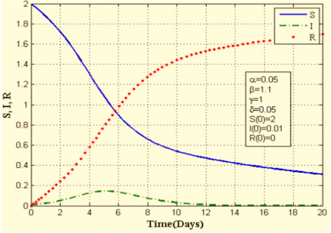
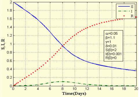
Figure 9 demonstrates the impact of isolation on the progression of epidemic transmission over time. The rate of isolating infected individuals plays a crucial role in curbing the spread of the coronavirus within the population. Notably, it can be observed (Figures 9(a), 9(b), and 9(c)) that as the rate of isolation decreases, the duration of the disease persists for a longer period. However, the fraction of infected individuals weakens over time.
(a)
(b)
(c)
Figure 8. Epidemic temporal evolution for different values of I (0): containment and isolation case
(a)
(b)
(c)
(d)
Figure 9. Isolation effects on the epidemic time evolution
In conclusion, it is important to acknowledge that obtaining accurate information regarding the evolution of the pandemic is challenging due to various factors, including the fluctuating number of tests conducted each day and the detection of individuals in contact with infected persons. Without comprehensive data on the real progression of the pandemic, particularly concerning asymptomatic individuals, estimating its parameters becomes a daunting task that requires further investigation in future studies.
The results show that it is possible to stop the spread of disease (or extinguish the endemic equilibrium) by correctly choosing the parameters that govern social and governmental behaviour. In the analysis that has been carried out, we conclude the main results.
In the analysis that has been carried out, the main results are concluded:
- The evolution of the reproduction number for the SIR model, has been extended to include the contribution of confinement and isolation (alpha and delta).
- This approach perfectly integrates social dynamics into the epidemiological model and considerably broadens understanding their interactions.
- The values of the transmissibility parameter and therefore the reproduction number (R0) suffered a significant reduction with the response approximately 14 days after the first incidence.
- The analysis predicts that an appropriate combination of the response to this protocol would effectively stop pandemics such as COVID-19.
The finding would support an argument to expand this protocol that stronger government actions and policies such as quarantines, wearing masks, vaccinations, social distancing and improving public perception could be essential to fight against the spread of COVID-19.
[1] Coronavirus. SARS-CoV-2.png| coronavirus. SARS - CoV-2. www.ncbi.nlm.nih.gov/ pmc/artcles/PMC7489918/.
[2] Lounis, M., Raeei, M.A. (2021). Estimation of epidemiological indicators of COVID-19 in Algeria with an SIRD model. Eurasian Journal of Medicine and Oncology, 5(1): 54-58. https://doi.org/10.14744/ejmo.2021.35428
[3] Anderson, S.C., Edwards, A.M., Yerlanov, M., Mulberry, N., Stockdale, J.E., Iyaniwura, S.A., Falcao, R.C., Otterstatter, M.C., Irvine, M.A., Janjua, N.Z., Coombs, D., Colijn, C. (2020). Quantifying the impact of COVID-19 control measures using a Bayesian model of physical distancing. PLoS Computational Biology, 16(12): e1008274. https://doi.org/10.1371/journal.pcbi.1008274
[4] Kucharski, A.J., Russell, T.W., Diamond, C., et al. (2020). Early dynamics of transmission and control of COVID-19: A mathematical modelling study. The Lancet Infectious Diseases, 20(5): 553-558. https://doi.org/10.1016/S1473-3099(20)30144-4
[5] David, R., Mishra, K., Gilbert, E.R., Mirza, K.M., Hendler, S. (2022). Indolent T-cell lymphoproliferative disease: A rare case of a benign lymphoma of the gastrointestinal tract with extra-gastrointestinal involvement. ACG Case Reports Journal, 9(10): e00879. https://doi.org/10.14309/crj.0000000000000879
[6] Musa, R., Ezugwu, A.E., Mbah, G.C. (2020). Assessment of the impacts of pharmaceutical and non-pharmaceutical intervention on COVID-19 in south Africa using mathematical model. MedRxiv, 2020-11. https://doi.org/10.1101/2020.11.13.20231159
[7] Peter, O.J., Shaikh, A.S., Ibrahim, M.O., Nisar, K.S., Baleanu, D., Khan, I., Abioye, A.I. (2021). Analysis and dynamics of fractional order mathematical model of COVID-19 in Nigeria using Atangana-Baleanu operator. Computers, Materials and Continua, 66(2): 1823-1848. https://doi.org/10.32604/cmc.2020.012314
[8] Peter, O.J., Qureshi, S., Yusuf, A., Al-Shomrani, M., Idowu, A.A. (2021). A new mathematical model of COVID-19 using real data from Pakistan. Results in Physics, 24: 104098. https://doi.org/10.1016/j.rinp.2021.104098
[9] Ndaïrou, F., Area, I., Nieto, J.J., Torres, D.F. (2020). Mathematical modeling of COVID-19 transmission dynamics with a case study of Wuhan. Chaos, Solitons & Fractals, 135: 109846. https://doi.org/10.1016/j.chaos.2020.109846
[10] Serhani, M., Labbardi, H. (2021). Mathematical modeling of COVID-19 spreading with asymptomatic infected and interacting peoples. Journal of Applied Mathematics and Computing, 66(1-2): 1-20. https://doi.org/10.1007/s12190-020-01421-9
[11] Iyaniwura, S.A., Rabiu, M., David, J.F., Kong, J.D. (2021). Assessing the impact of adherence to non-pharmaceutical interventions and indirect transmission on the dynamics of COVID-19: A mathematical modelling study. Mathematical Biosciences and Engineering, 18(6): 8905-8932. https://doi.org/10.3934/mbe.2021439
[12] Ivorra, B., Ferrández, M.R., Vela-Pérez, M., Ramos, A.M. (2020). Mathematical modeling of the spread of the coronavirus disease 2019 (COVID-19) taking into account the undetected infections. The case of China. Communications in Nonlinear Science and Numerical Simulation, 88: 105303. https://doi.org/10.1016/j.cnsns.2020.105303
[13] Zhong, H., Wang, W. (2020). Mathematical analysis for COVID-19 resurgence in the contaminated environment. Mathematical Biosciences and Engineering, 17(6): 6909-6927. https://doi.org/10.3934/mbe.2020357
[14] Aldila, D. (2020). Cost-effectiveness and backward bifurcation analysis on COVID-19 transmission model considering direct and indirect transmission. Communications in Mathematical Biology and Neuroscience, 2020: 49.
[15] Tuite, A.R., Fisman, D.N., Greer, A.L. (2020). Mathematical modelling of COVID-19 transmission and mitigation strategies in the population of Ontario, Canada. CMAJ, 192(19): E497-E505. https://doi.org/10.1503/cmaj.200476
[16] Cao, J., Jiang, X., Zhao, B. (2020). Mathematical modeling and epidemic prediction of COVID-19 and its significance to epidemic prevention and control measures. Journal of Biomedical Research & Innovation, 1(1): 1-19.
[17] Liu, Z., Magal, P., Seydi, O., Webb, G. (2020). A COVID-19 epidemic model with latency period. Infectious Disease Modelling, 5: 323-337. https://doi.org/10.1016/j.idm.2020.03.003
[18] Behring, B.M., Rizzo, A., Porfiri, M. (2021). How adherence to public health measures shapes epidemic spreading: A temporal network model. Chaos: An Interdisciplinary Journal of Nonlinear Science, 31(4): 043115. https://doi.org/10.1063/5.0041993
[19] Alagoz, O., Sethi, A.K., Patterson, B.W., Churpek, M., Safdar, N. (2021). Effect of timing of and adherence to social distancing measures on COVID-19 burden in the United States: A simulation modeling approach. Annals of Internal Medicine, 174(1): 50-57. https://doi.org/10.7326/M20-4096
[20] Van den Driessche, P., Watmough, J. (2002). Reproduction numbers and sub-threshold endemic equilibria for compartmental models of disease transmission. Mathematical Biosciences, 180(1-2): 29-48. https://doi.org/10.1016/S0025-5564(02)00108-6
[21] Diekmann, O., Heesterbeek, J.A.P., Metz, J.A. (1990). On the definition and the computation of the basic reproduction ratio R 0 in models for infectious diseases in heterogeneous populations. Journal of Mathematical Biology, 28: 365-382. https://doi.org/10.1007/BF00178324
[22] van den Driessche, P., Watmough, J. (2008). Further Notes on the Basic Reproduction Number. In: Brauer, F., van den Driessche, P., Wu, J. (eds) Mathematical Epidemiology. Lecture Notes in Mathematics, vol 1945. Springer, Berlin, Heidelberg. https://doi.org/10.1007/978-3-540-78911-6_6
[23] Perasso, A. (2018). An introduction to the basic reproduction number in mathematical epidemiology. ESAIM: Proceedings and Surveys, 62: 123-138. https://doi.org/10.1051/proc/201862123