Haryono Setiyo Huboyo*![]() | Okto Risdianto Manullang | Budi P Samadikun
| Okto Risdianto Manullang | Budi P Samadikun![]()
© 2023 IIETA. This article is published by IIETA and is licensed under the CC BY 4.0 license (http://creativecommons.org/licenses/by/4.0/).
OPEN ACCESS
Control of short-lived climate forcers (SLCF) is very crucial because it has quicker impact and more visible benefits in the short-term than control of carbon dioxide. For this reason, this research is aimed at estimating the level of SLCF (black carbon/BC, methane, and ozone) in the atmosphere, their impact and associated health risk (of certain SLCF). We measured BC at PM2.5, ground level ozone in 24h, and CH4, N2O and CO2 in five different sites in different land use categories. We also distributed questionnaires to vulnerable populations in the study area. The concentration of BC was in the range of 2.42-5.52 ug/m3. The proportion of BC in PM2.5 is between 4.9% and 12.74%. Ambient methane concentrations were higher in the morning than in the afternoon. Likewise, the oxidant concentration of O3, N2O, and CO2 showed that results of measurement were higher in the morning than in the afternoon. The average concentration ratio of short-term to long-term greenhouse gas (CH4: N2O: CO2) is 4.9:1:1304. In terms of health risk, Estimated Attribute Proportion (AP) resulting from BC is within 1.1% and 7.48%. Mitigation of short-term GHG pollutant emission sources would be in line with long-term GHG pollutant mitigation.
emissions, GHG, global warming, urban areas, SLCF
Human activities are responsible for the main changes in the atmosphere including the composition of long-lived and short-lived GHGs. Long-lived GHGs usually have life spans of more than 8 years in the atmosphere, while short-lived GHGs or short-lived climate forcers (SLCF) could have lifetimes of only a few weeks [1]. Black carbon (BC), tropospheric ozone, and methane are among the SLCF capable of degrading the ambient air quality by disturbing the Aerosol optical depth [2]. BC reduces light and reflects it back into space. This ability depends on its reflectivity beneath surfaces and its mixture with particulate matter. Methane could ordinarily be categorized as a long-lived greenhouse gas; however, due to relatively warming the climate it could also be categorized as SLCF [3]. Methane, indirectly, is also a precursor pollutant for tropospheric ozone. Tropospheric ozone is a strong oxidant that is harmful to public health and increases the disease burden. Several SLCF significantly contribute to the rising global temperature. Many studies have revealed the following as contributors of ambient BC: biomass burning and traffic [4] , forest fire [5], domestic stove [6] and fired coal [7]. In urban areas, the main contributor of BC was fossil fuel burning, while in rural area, the main contributor of BC was biomass burning. More than 80% of global BC emission was attributed to open biomass and solid fuel burning. From many studies, the ambient PM2.5 contains about 10% BC [8, 9, 10]. Global BC emission is estimated at 8 TgC/year [11]. Indonesia contributes 6% of total BC in Asia, the third largest in Asia [12]. The ambient methane (CH4) was most times analyzed with other GHGs such as CO2 and N2O [13, 14]. Methane emission and mitigation are generally associated with the petroleum (oil and gas) industry [15]. Global methane emission was estimated at 344 Gg in 2017 [16] while anthropogenic emissions of methane accounted for about half of total CH4 emissions.
Several climate change studies have shown that rapid response to SLCF could significantly reduce short-term global temperatures by 40% to 45% in a decade [11], prevent potential global temperature rise of 0.6°C by 2050 [17], prevent more than 0.84 °C potential global temperature rise by 2070 [11], and reduce climate cycles, particulate matter (PM2.5) and ozone pollution for human health, agriculture, and ecosystems [18, 19]. This effectiveness can be achieved if SLCF control is carried out in tandem with the maximum control carried out on the main long-term contributor, (CO2) [11].
Many interventions are intended to mitigate rise in short-term global temperature [20]. The initial steps of mitigation start by inventorying emissions distribution and identifying the main contributing sources of SLCF from anthropogenic sources [21]. Emission inventory of conventional air pollutants was recently conducted in Semarang City of Indonesia [22, 23]. It is hoped that same will be done for SLCF to enable mitigation action for SLCF. The mitigation action itself, going by carbon dioxide mitigation at the national level has challenges of validating the quantitative results of such mitigation action. For instance, after subjecting previous researches to verification processes, it was hard to find any reliable national mitigation action for reduction of greenhouse gases in the transportation sector [24]. Above all, the level of short-term greenhouse gases in Indonesia is quite unprecedented for identifying the status of ambient SLCF concentration. This research is intended to determine the magnitude of SLCF pollutants in the city of Semarang and health risks associated with certain SLCF.
2.1 Site sampling
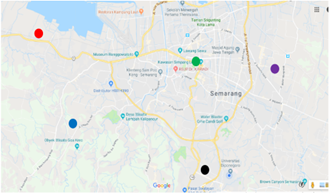
Five locations cutting across industrial, commercial, residential, education, and relatively remote areas were selected for sampling. Ambient particulate matter with size aerodynamic diameter less than 2.5 microns (PM2.5) was sampled in these sites. Figure 1 shows the location where PM2.5 24h measurements were conducted, and detailed coordinates are presented in Table 1. We took measurements three times during the dry season i.e., 18–23, August 2018; 6–11, September 2018 and 12–17, September 2018. During this time, very light precipitation occurred at the end of the sampling period (Figure 1).
Figure 1. Sampling point measurement
Table 1. Site location for measurement
|
No |
Site Name |
Coordinates |
Remark |
|
1 |
Tugu |
06° 58' 02, 96" S, 110° 20' 14, 45" E |
Industrial area |
|
2 |
Pleburan |
06° 59' 39, 89" S, 110° 25' 28, 11" E |
Commercial area |
|
3 |
Pedurungan |
07° 00' 21, 62" S, 110° 28' 23, 85" E |
Residential area |
|
4 |
Tembalang |
07° 22' 55, 51" S, 110° 25' 13, 28" E |
Education area |
|
5 |
Gunung Pati |
07° 05' 17, 12" S, 110° 23' 08, 60" E |
Remote area |
2.2 PM2.5 sampling and lab analysis
We sampled PM2.5 for 24h using PM2.5 high volume sampler monitoring device, Staplex at a constant flow rate of 1100 L/min. Quartz filter, Whatman, was used for sampling. After sampling, the filters were kept below 20 °C with RH < 50%. Co-located blank filters were provided during the sampling exercise. The filters were then weighed with a Mettler Toledo microbalance.
The EEL Reflectometer (EEL 23 M) was used to quantify BC concentration in 19.625 cm2 of the total filter area. We analyzed each filter twice for BC at the National Nuclear Power Agency laboratory in Bandung City to ascertain low variability of BC in the filters. For tropospheric ozone (O3) parameter, we used an impinger equipped with a vacuum pump at a constant flow rate of 0.5 L/min for 1h. We carried out measurement twice i.e., 10 A.M. and 2 P.M., to represent peak O3 ambient concentration. The reference method used for tropospheric ozone measurement was Indonesian National Standard (SNI) No. 19-7119.8-2005. To identify other potential greenhouse gases, we took grab ambient methane (CH4), dinitro oxides (N2O), and CO2 measurements by collecting them with a Zefon USA 1L tedlar bag. The ambient air was sampled using a small pump (Aircheck 224-44XR) at a constant flow rate of 0.1 L/min for about 10 minutes. Like the tropospheric ozone measurement, other GHGs measurements were done twice i.e., 10 A.M. and 2 P.M. After sampling, gas chromatography (Shimadzu GC-14A) was used to quantify CH4, N2O and CO2 in the tedlar bags at the Agricultural Research Center of Pati Regency, Indonesia. Gas chromatography used 3 detectors namely FID, ECD and TID detectors for each gas CH4, N2O and CO2. Gas samples from tedlar bags were taken 2 mL and analyzed by GC for CH4, N2O and CO2 for 5, 7 and 5 minutes running respectively
2.3 Questionnaire survey
Simultaneously with the measurement activities, we collected secondary data to identify the population characteristics. We collected data in details on the total population of each study area, number of vulnerable population (aged ≤5 and ≥30 years) in each study area and area of the measurement site. Then the data was analyzed with AirQ+ to produce Estimated Attributable Population or the estimate of population experiencing health problems categorized by types of health disorders. Questionnaires were also administered to 500 people within vulnerable populations in each study area. The questionnaires were designed in written and/or unwritten forms. Questionnaires were administered in urban villages within a kilometer radius of the air quality measurement sampling site. Slovin’s Formula was used to calculate the sample size of each site, which amounted to a total of 500 respondents; calculate the number of samples in a sizable population and measure the proportion of each population.
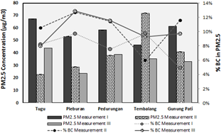
The concentration of PM2.5 was twice recorded to have exceeded the air quality standard, firstly in Tugu and Gunung Pati and secondly in Tembalang. The third measurement of PM2.5 concentration was also below the quality standard. On the average, the PM2.5 results were somewhat lower than those of Jakarta City [25] i.e., between 46 and 77 ug/m3 and higher those of Bandung City [26] i.e., about 15 ug/m3. The first and second measurements were done at the end of the dry season while there was partial rainfall when the third measurement was done (Figure 2).
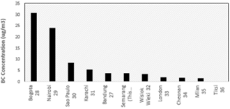
Recorded BC concentrations are much lower (depicted in Figure 3) than other ambient BC concentrations in other countries like Bogota, Colombia [27], Nairobi, Kenya [28], Sao Paulo, Brazil [29] and Karachi, Pakistan [30] that had ambient black carbon concentration in the range 5.5 – 30.7 µg/m3. Several measurements in these countries located close to big road to represent near roadside thus showed high ambient BC. However, Indonesian ambient BC concentrations are higher than those of European countries and Asian developed country for example Wislok Wielki, Poland [31], London, UK [32], Cheonan, South Korea [33], Milan, Italy [34], Tiksi, Russia [35] which had ambient black carbon concentration in the range 0.17 – 3.48 µg/m3.
Figure 2. Percentage of BC in PM2.5 concentration
Figure 3. Comparison of ambient BC concentration with other studies
3.1 Ozon, methane, dinitrooxide, carbon dioxide
As featured in Figure 4, ozone concentration in the Tembalang area (education area) has the highest concentration compare to other land use areas (industrial, commercial, residential dan remote area). The ratio of ozone concentration in the morning to ozone in the afternoon ranges from 0.6 to 1.6, which the highest ratio was in the Tembalang area (educational area). The average ambient O3 concentration detected was far lower than that in the Indonesian standard (117 ppb or 235 µg/m3). While the CH4 concentration ratio between morning and afternoon ranges from 0.85 to 1.2 where the highest occurs in commercial areas. As for N2O, the concentration ratio in the morning and afternoon ranges around 0.9 - 1.0 where the highest in the industrial area although the difference with other locations is very slight. The N2O has the highest uncertainty measurement results as indicated by the deviation from the conceived standard deviation.
Note: A: afternoon (2 PM), M: morning (10 AM)
Figure 4. Concentration of ground level ozone, methane, nitrous oxide and carbon dioxide (morning-afternoon)
Likewise, it condition also occurs for ambient CO2 concentrations where the ratio of the concentration in the morning and afternoon is around 1.0 - 1.09. Visually, the results are displayed as in Figure 4.
3.2 Questionnaire results
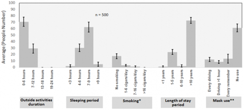
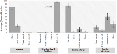
We had 100 respondents among vulnerable people in each district (totaling 500 respondents), and the results are depicted in Figure 5. Among 100 vulnerable respondents in all of these sites approximately 14 - 16% are toddlers (1 - 5 years old). The respondents have lived in this area for over 10 years. Thus, majority of the respondents live in their own property. The average respondent spent less than 1/4 of the day outside the house because they work informally and formally and therefore spend a lot of time indoors; so the possibility of exposure to ambient air pollutants is relatively small. The sleeping habits of the respondents were also quite good (7-8 hours sleep).
Note: * not all respondent respond well to smoking
** mask is used while driving two wheels vehicle
Note: * health related to air pollution exposure
Figure 5. Average questionnaire results from 5 locations
The questionnaire result unrealistically showed that smoking habits of respondents was less than 50% because they do not smoke on the average. The use of masks while driving two-wheeled vehicles is relatively minimal at 12% while non-use of masks is 60%. Masks are usually worn to reduce exposure to smoke while driving two-wheeled vehicles in Indonesia.
80% of the surveyed population was not accustomed to exercise/sports while the remaining 20% do sports once a week. Lack of exercise can reduce the body’s resistance to air pollution. Nevertheless, results showed that more than 90% did not suffer diseases related to air pollution, and the variation between districts was relatively small. This corresponds with the aspect of the results showing that 77%-97% of respondents did not have an allergy to smoke, while approximately 10% was allergic to vehicle smoke. The average respondent had high medical awareness, knowing to visit a doctor when feeling sick while 26% of respondents did not see a doctor when sick.
50% of respondents believed that the current air is of medium quality; and 30% consider the quality good. While 60% of respondents do not feel disturbed by the air quality, 25% feel a little disturbed. 40% of respondents reported feeling discomfort between 11 A.M. and 3 P.M. This time range is clearly not the peak of air pollution resulting from motorized vehicles. The peak periods for vehicles are between 7 A.M. and 8 A.M. and between 4 P.M. and 6 P.M. Despite this, about 84% of the respondents still consider the transportation sector the main contributor to air pollution followed by 10% who believe it is biomass burning.
The percentage of BC content in PM2.5 ranged from 4.9% to 12.74%. In majority of the measurements, BC content in PM2.5 was more than 7.5%, a clear violation of WHO standard. The highest percentage of BC consistently occurred in commercial areas (i.e., in Pleburan). This is probably due to the high number of vehicles using diesel fuel. Based on recent emission inventory, vehicles in urban areas account for almost 70% of NOx pollutants in Semarang City. It is clear that ambient BC concentrations in developing countries are much higher than those at developed countries either in Europe or in Asia, therefore much efforts should be done for mitigating BC emission at developed countries level.
The concentration of ambient greenhouses is generally lower in the afternoon than in the morning, but the difference is not very significant. Generally the O3 oxidant concentration was higher in the morning than in the afternoon. The Tembalang area, close to areas with many vehicles, had a high ambient ozone concentration, which indicates NOx as the precursor to ozone in this area. Overall, the CH4 concentration was fairly low, this is due to the main source of methane gas i.e anaerobic decay of organic material, was not present in the area of measurement. The concentration of N2O varied considerably between Gunung Pati and Pleburan, but is quite high or low at specific times. This indicates that the source of N2O was not ascertained, and it occasionally appeared as a source of pollutants in certain locations. Variations in CO2 concentration also occurred, but in the Tugu area, it was consistently high in the morning. Tugu area is an area that has quite a lot of industrial activities; so the possibility of CO2 emissions is quite high.
Calculated average greenhouse gas ratio in measurement samples were (CH4:N2O:CO2) = 4.9:1:1304. When we examine the results, it is observed that the concentration of CO2 remains a major contributing factor to global warming, followed by N2O and CH4. Mitigation of these pollutant emission sources needs to integrate both long-term and short-term GHG emission sources. Based on emission inventory, in 2017, the total consumption of LPG in the domestic sector in Semarang City was 48,532 tons and these produce a total SCLF emissions of 0.537 tons/year and 11,538 tons/year for BC and CH4 respectively [36]. This corresponds with CO2 emissions of 145,611 tons/year and N2O emission of 230.76 tons/year. Emissions in transport areas, based on VKT data combined with active vehicles data, reached 178.23 tons/year, 802.52 tons/year, and 88.78 tons/year for BC, CH4, and N2O respectively. This transportation sector produces total CO2 emissions of 2,123,302 tons/year (almost 15 times that of the domestic sector). Thus, it is important to control the main sources of SLCF and long term GHGs (i.e CO2 and N2O). Mitigation of short-term and conventional GHG pollutant emission sources could be done simultaneously because they have the same sources i.e domestic and transport sector.
AirQ+ calculation showed that Gunung Pati district was the biggest population with health risk although the population density showed the least. The estimated health risk calculation results, as depicted in Table 2, show that the Estimated Attribute Proportion (AP) due to ambient PM2.5 is highest in Gunung Pati, while the highest number of cases is in the Banyumanik district. In Semarang City, 4.6%–7.4% of HA–RD, 2.2%–3.6% of HA–CVD and 3.03%–4.9% of mortality were attributed to PM2.5. The estimated health risk is much higher in Indonesia than Italy [37] and a little bit lower than Iran [38].
The least AP and cases due to PM2.5 were in Tugu district; while for BC, the highest AP was located at Pedurungan district at 7.48%. Pedurungan dan Banyumanik is a land reserved for settlement. Thus, high health risk attributed to PM2.5 and BC should be mitigated accordingly. Based on AERMOD modeling studies recently, the dispersion of pollutants derived from the transportation sector were concentrated in the center, East, and South of Semarang City [36]. These areas include South Semarang, Pedurungan, and Banyumanik. Reducing the use of private cars/motorcycles is highly recommended since the main source of BC in urban areas is the transportation sector. Therefore, simultaneous SLCF and conventional GHG could be mitigated by handling mitigation in the transportation sector.
The Air Q+ model requires relatively simple data as an input. In developing countries, that air quality data is adequate in urban areas and population censuses are widely available for population statistics, Air Q+ could be delivered. However, there is a weakness of this method because there is no unaffected control population as in case-control studies or case-crossover studies so that the resulting impact is not necessarily site-specific.
Table 2. Health endpoints of PM2,5 and BC
|
District |
Health Endpoint, Estimated Attribute Proportion (AP) Due to PM2.5 |
Health Endpoint, Estimated Attribute Proportion (AP) Due to BC |
||
|
HA-RD |
HA-CVD |
Mortality |
||
|
Tugu |
6,32% |
3,09% |
4,15% |
2,64% |
|
Case number |
435 |
213 |
286 |
182 |
|
Pedurungan |
4,63% |
2,26% |
3,03% |
7,48% |
|
Case number |
691 |
337 |
452 |
1116 |
|
South Semarang |
6,38% |
3,12% |
4,19% |
5,85% |
|
Case number |
2248 |
1099 |
1476 |
680 |
|
Gunungpati |
7,46% |
3,66% |
4,91% |
1,11% |
|
Case number |
1995 |
979 |
1313 |
474 |
|
Banyumanik |
6,39% |
3,13% |
4,20% |
1,62% |
|
Case number |
2862 |
1402 |
1881 |
1000 |
Notes:
HA-RD: Hospital admissions, respiratory disease
HA-CVD: Hospital admission, CVD (including stroke)
Mortality: Mortality all (natural) causes (adults age 30+ years)
The results of the measurement of BC as one of the SLCF show that it is in the range of 2.42 and 5.52 ug/m3. This concentration is classified as moderate quantity. The proportion of BC in PM2.5 is between 4.9% and 12.74%. Methane concentration in the morning was higher than in the afternoon, but the difference was not too significant. Likewise, oxidant concentration of O3, N2O, and CO2 was higher in the morning than in the afternoon. The ratio of SLCF to long-term greenhouse gas (CH4: N2O: CO2) = 4.9:1:1304. Current air pollution status in the study area is still considered good. Estimated AP due to ambient PM2.5 in Semarang City is 4.6%–7.4% for HA–RD, 2.2%–3.6% for HA–CVD, and 3.03%–4.9% for mortality. Estimated AP due to BC falls within 1.1% and 7.48%. Mitigation of short-term and conventional GHG pollutant emission sources could be done simultaneously.
This study was supported by Directorate General of Research and Development Reinforcement, Ministry of Research, Technology and Higher Education, Republic of Indonesia (Grant No.: 101-75/UN7.P4.3/PP/2018).
[1] Shindell, D., Ramanathan, V., Raes, F., Cifuentes, L., Kim Oanh, N.T. (2012). Integrated assessment of black carbon and tropospheric ozone: Summary for decision makers. United Nations Environment Programme.
[2] Hu, A., Xu, Y., Tebaldi, C., Washington, W.M., Ramanathan, V. (2013). Mitigation of short-lived climate pollutants slows sea-level rise. Nature Climate Change, 3(8): 730-734. https://doi.org/10.1038/nclimate1869
[3] Aamaas, B., Berntsen, T.K., Fuglestvedt, J.S., Shine, K.P., Bellouin, N. (2016). Regional emission metrics for short-lived climate forcers from multiple models. Atmospheric Chemistry and Physics, 16(11): 7451-7468. https://doi.org/10.5194/acp-16-7451-2016
[4] Singh, S., Tiwari, S., Hopke, P.K., Zhou, C., Turner, J. R., Panicker, A.S., Singh, P.K. (2018). Ambient black carbon particulate matter in the coal region of Dhanbad, India. Science of the Total Environment, 615: 955-963. https://doi.org/10.1016/j.scitotenv.2017.09.307
[5] Evans, M., Kholod, N., Kuklinski, T., Denysenko, A., Smith, S.J., Staniszewski, A., Bond, T.C. (2017). Black carbon emissions in Russia: A critical review. Atmospheric Environment, 163: 9-21. https://doi.org/10.1016/j.atmosenv.2017.05.026
[6] Garland, C., Delapena, S., Prasad, R., L'Orange, C., Alexander, D., Johnson, M. (2017). Black carbon cookstove emissions: A field assessment of 19 stove/fuel combinations. Atmospheric Environment, 169: 140-149. https://doi.org/10.1016/j.atmosenv.2017.08.040
[7] Kucbel, M., Corsaro, A., Švédová, B., Raclavská, H., Raclavský, K., Juchelková, D. (2017). Temporal and seasonal variations of black carbon in a highly polluted European city: Apportionment of potential sources and the effect of meteorological conditions. Journal of Environmental Management, 203: 1178-1189. https://doi.org/10.1016/j.jenvman.2017.05.038
[8] Baumgardner, D., Kok, G.L., Raga, G.B. (2007). On the diurnal variability of particle properties related to light absorbing carbon in Mexico City. Atmospheric Chemistry and Physics, 7(10): 2517-2526. https://doi.org/10.5194/acp-7-2517-2007
[9] Chow, J.C., Watson, J.G., Lowenthal, D.H., Chen, L.W.A., Motallebi, N. (2011). PM2. 5 source profiles for black and organic carbon emission inventories. Atmospheric Environment, 45(31): 5407-5414. https://doi.org/10.1016/j.atmosenv.2011.07.011
[10] Briggs, N.L., Long, C.M. (2016). Critical review of black carbon and elemental carbon source apportionment in Europe and the United States. Atmospheric Environment, 144: 409-427. https://doi.org/10.1016/j.atmosenv.2016.09.002
[11] IPIECA. (2014). Understanding short-lived climate forcers.
[12] USAID. (2010). Black Carbon Emissions in Asia: Sources, Impacts, and Abatement Opportunities, 43: 515-516.
[13] Folberth, G.A., Rumbold, S.T., Collins, W.J., Butler, T.M. (2012). Global radiative forcing and megacities. Urban Climate, 1: 4-19. https://doi.org/10.1016/j.uclim.2012.08.001
[14] Hooghiem, J.J., de Vries, M., Been, H.A., Heikkinen, P., Kivi, R., Chen, H. (2018). LISA: A lightweight stratospheric air sampler. Atmospheric Measurement Techniques, 11(12): 6785-6801. https://doi.org/10.5194/amt-11-6785-2018
[15] Evans, M., Roshchanka, V. (2014). Russian policy on methane emissions in the oil and gas sector: A case study in opportunities and challenges in reducing short-lived forcers. Atmospheric Environment, 92: 199-206. https://doi.org/10.1016/j.atmosenv.2014.04.026
[16] Polag, D., Keppler, F. (2019). Global methane emissions from the human body: Past, present and future. Atmospheric Environment, 214: 116823. https://doi.org/10.1016/j.atmosenv.2019.116823
[17] Myhre, G., Samset, B.H., Schulz, M., Balkanski, Y., Bauer, S., Berntsen, T.K., Zhou, C. (2013). Radiative forcing of the direct aerosol effect from AeroCom Phase II simulations. Atmospheric Chemistry and Physics, 13(4): 1853-1877. https://doi.org/10.5194/acp-13-1853-2013
[18] Kirtman, B., Power, S.B., Adedoyin, A.J., Boer, G.J., Bojariu, R., Camilloni, I., Wang, H.J. (2013). Near-term climate change: projections and predictability. Climate Change 2013: The Physical Science Basis. IPCC Working Group I Contribution to AR5., 953-1028.
[19] Zha, S., Cheng, T., Tao, J., Zhang, R., Chen, J., Zhang, Y., Du, J. (2014). Characteristics and relevant remote sources of black carbon aerosol in Shanghai. Atmospheric research, 135: 159-171. https://doi.org/10.1016/j.atmosres.2013.09.002
[20] Akimoto, H., Kurokawa, J.I., Sudo, K., Nagashima, T., Takemura, T., Klimont, Z., Suzuki, K. (2015). SLCP co-control approach in East Asia: Tropospheric ozone reduction strategy by simultaneous reduction of NOx/NMVOC and methane. Atmospheric Environment, 122: 588-595. https://doi.org/10.1016/j.atmosenv.2015.10.003
[21] Rogelj, J., Schaeffer, M., Meinshausen, M., Shindell, D.T., Hare, W., Klimont, Z., Schellnhuber, H.J. (2014). Disentangling the effects of CO2 and short-lived climate forcer mitigation. Proceedings of the National Academy of Sciences, 111(46): 16325-16330. https://doi.org/10.1073/pnas.1415631111
[22] Bunawati, T.T., Huboyo, H.S. Samadikun, B.P. (2017). Conventional polution emission estimation (SOx, Box, CO, and PM) from the private vehicle based on interbational vehicle emission model in Several roads of Semarang City. Jurnal Teknik Lingkungan, 6: 1-12.
[23] Chaerunnisa, L.H., Samadikun, B.P. Huboyo, H.S. (2017). Estimation of conventional air pollutants (SOx, NOx, CO, AND PM) from public transport based on international vehicle emission (IVE) method in Semarang city road. Jurnal Teknik Lingkungan, 6: 1-17.
[24] Huboyo, H., Wibowo, H., Sari, W.R. (2018). Green House Gases (GHG’s) Emission Reduction Measures and Verification Challenge at Transport Sector. In MATEC Web of Conferences, Bali, Indonesia, EDP Sciences, pp. 01027. https://doi.org/10.1051/matecconf/201815901027
[25] Muliane, U., Lestari, P. (2011). Pemantauan kualitas udara ambien daerah padat lalu lintas dan komersial DKI Jakarta: analisis konsentrasi PM2, 5 dan black carbon. Jurnal Teknik Lingkungan, 17(2): 178-188.
[26] Lestiani, D.D., Santoso, M., Hidayat, A. (2007). Karakteristik Black Carbon Partikulat Udara Halus PM2, 5 di Bandung dan Lembang 2004-2005. Jurnal Sains dan Teknologi Nuklir Indonesia, 9: 89-94.
[27] Betancourt R, Galvis B, Balachandran S, Ramos-Bonilla J, Sarmiento O, Gallo-Murcia S, Contreras Y (2017) Exposure to fine particulate, black carbon, and particle number concentration in transportation microenvironments. Atmos Environ 157, 135-145.
[28] Gataria M et al. (2019). High airborne black carbon concentrations measured near roadways in Nairobi, Kenya. Transport Res Transport Environ 68, 99-109.
[29] Targino AC, Krecl P, Filho JED, Segura JF, Gibson MD (2018) Spatial variability of on-bicycle black carbon concentrations in the megacity of São Paulo: A pilot study. Environ Pollut 242, 539-43.
[30] Bibi, S, Alam K, Chishtie F, Bibi H, Rahman S (2017) Temporal variation of Black Carbon concentration using Aethalometer observations and its relationships with meteorological variables in Karachi, Pakistan. J Atmos Sol Terr Phys 157–158, 67-77.
[31] Chilinski MT, Markowicz KM, Markowicz J (2016) Observation of vertical variability of black carbon concentration in lower troposphere on campaigns in Poland, Atmos Environ 137, 155-170.
[32] Singh V, Ravindra K, Sahu L, Sokhi R (2018) Trends of atmospheric black carbon concentration over the United Kingdom. Atmos Environ 178, 148-57.
[33] Lee J, Yun J, Kim K (2016). Monitoring of black carbon concentration at an inland rural area including fixed sources in Korea. Chemosphere 143, 3-9.
[34] Mousavi A et al. (2019) Source apportionment of black carbon (BC) from fossil fuel and biomass burning in metropolitan Milan, Italy. Atmos Environ 203, 252-261.
[35] Popovicheva O, Diapouli E, Makshtas A, Shonija N, Manousakas M, Saraga D, Uttal T, Eleftheriadis K (2019) East Siberian Arctic background and black carbon polluted aerosols at HMO Tiksi, Sci Total Environ 655, 924-38.
[36] Huboyo, H., Samadiku, B., Manullang, O. (2021). Emission comparison of short lived climate forcers over long term greenhouse gases from domestic and transport sector in Semarang city. Materials Science and Engineering, 1108(1): 012008. https://doi.org/10.1088/1757-899X/1108/1/012008
[37] De Marco, A., Amoatey, P., Khaniabadi, Y.O., Sicard, P., Hopke, P.K. (2018). Mortality and morbidity for cardiopulmonary diseases attributed to PM2. 5 exposure in the metropolis of Rome, Italy. European Journal of Internal Medicine, 57: 49-57. https://doi.org/10.1016/j.ejim.2018.07.027
[38] Asl, F.B., Leili, M., Vaziri, Y., Arian, S.S., Cristaldi, A., Conti, G.O., Ferrante, M. (2018). Health impacts quantification of ambient air pollutants using AirQ model approach in Hamadan, Iran. Environmental Research, 161: 114-121. https://doi.org/10.1016/j.envres.2017.10.050