Kai Wei | Qiandeng Li | Jiacui Luan | Minggang Liu | Xingyi Wang*
© 2020 IIETA. This article is published by IIETA and is licensed under the CC BY 4.0 license (http://creativecommons.org/licenses/by/4.0/).
OPEN ACCESS
Drilling safety is the foundation for the safe and efficient development of oil and gas resources. However, drilling accidents (e.g. blowout, lost circulation and borehole instability) often occur due to the complex geological conditions, especially in deep wells, ultra-deep wells and offshore oil and gas wells. To prepare a targeted drilling plan and minimize drilling risks, the key is to grasp the accurate geological parameters of the target formation. However, drilling safety is seriously threatened by the numerous complex, stochastic, and uncertain factors in the target formation, as well as the errors in the formation parameters captured by the current techniques. This paper attempts to quantify drilling risk accurately, despite the uncertainty of drilling information, and make efficient use of geological parameters. For this purpose, the concept of formation matrix was put forward, and coupled with credibility to handle the inevitable errors in formation parameters. According to the mechanical mechanism of common drilling risks, a Monte-Carlo (MC) simulation method was established to calculate the probabilities of drilling risks. The proposed method was applied to evaluate the well kick risk of a well in Kekeya area of Tuha Basin. The results show that our method can accurately predict the drilling risks that conforms to the mechanical hazard mechanism, effectively integrate various drilling information, making them complement each other, and improve the characterization accuracy of formation matrix, thereby enhancing the reliability of drilling risk evaluation. The proposed method provides theoretical support for geological modeling and drilling risk evaluation.
drilling risks, formation matrix, credibility, risk probability, Monte-Carlo (M-C) simulation
Oil and gas companies invest about 20 billion USD annually in drilling. Over 15% of that investment is lost due to drilling accidents, which seriously dampens the benefits of oil and gas exploration and development. The typical drilling accidents include blowout, lost circulation and wellbore instability. Most of them arise from the complex geological conditions of drilling wells [1-3]. Therefore, it is of great importance to evaluate, monitor and manage drilling safety.
To prepare a targeted drilling plan and minimize drilling risks, the key is to grasp the accurate geological parameters of the target formation [4]. However, errors may occur in the prediction of these parameters, owing to the numerous complex, stochastic, and uncertain factors in the geological environment, plus the limited detection techniques of formation information. Hence, the geological parameters are often uncertain [5-7], making it difficult to quantify drilling risks.
Many scholars have attempted to evaluate drilling risk accurately, despite the uncertainty of drilling information. For example, Yasseri [8] screened the factors affecting drilling safety with the risk matrix, and ranked the risk factors through analytic hierarchy process (AHP). Khakzad et al. [9] evaluated the risks of drilling accidents, using the bow-tie model and Bayesian network (BN). Li et al. [10] created a knowledge base through knowledge integration, relied on the knowledge base to design the overall architecture of a drilling risk management system, and specified the construction of each submodule; the designed system is clear in logic and easy to implement, capable of identifying, evaluating, assessing and controlling drilling risks.
Through Monte-Carlo (MC) simulation, Wei [11, 12] set up a theoretical system for drilling risk evaluation, following the generalized stress and strength interference theory (GSSIT); Next, a real-time drilling risk monitoring method was developed based on backpropagation neural network (BPNN), according to the uncertainty of drilling monitoring parameters and their correlation with complex downhole accidents. Considering the interval distribution features of geological parameters, Guan et al. [13] proposed a non-probabilistic evaluation method of drilling risks.
With the aid of the BN, Bhandari et al. [14] conducted dynamic safety evaluation of pressure-controlled drilling and underbalanced drilling operations, and analyzed various potential risk factors. Charles et al. [15] identified uncertain geomechanical parameters for drilling engineering, and then created a drilling risk evaluation and control system, which predicts risks before drilling, monitors risks during drilling, and summarizes risks after drilling. Based on genetic backpropagation (BP) algorithm, Liang et al. [16] established an intelligent early diagnosis model of drilling overflow, realizing timely diagnosis of drilling overflow accidents.
The above studies show that geological information of drilling engineering is the only basis for understanding the target formation. The mastery of drilling information directly bears on the success or failure of drilling operations. For better evaluation of drilling risks, it is critical to characterize drilling information and improve data processing efficiency. The development of computer technology makes it possible to digitize the formation information in true three-dimensional (3D) space [17], giving a full and intuitive display of the formation attributes. This allows researchers to fully mine the digital formation information, and conduct scientific evaluation of drilling risks.
Considering the vague expression of geological information, this paper aims to digitize the fuzzy geological information of drilling engineering, which helps to better understand, express and represent geological bodies and geological environment. For this purpose, the concept of formation matrix was proposed, in the light of the similarity of multidimensional formation attributes and matrix [17], and a formation matrix with credibility was constructed based on stratigraphic sequence and probability statistics. Drawing on the GSSIT, an evaluation method was presented for drilling risks like well kick, lost circulation, differential pressure sticking, and collapse. After that, the risk probabilities of complex drilling accidents were solved by MC simulation, and the well sections prone to such accidents were identified. The proposed method provides guidance for wellbore structure design, drilling fluid density design and engineering construction.
Digital formation is a multidimensional concept involving various attributes, such as time, space, and formation parameters. For any point i in the static formation, the relevant attributes can be characterized by a matrix [xi, yi, zi, pi], where xi, yi, and zi are the spatial coordinates of the point, and pi is a physical attribute of that point.
For scientific management and application of digital formation information, the above characterization method was extended to the entire formation, creating the formation matrix. For a formation, the spatial coordinates and the said physical attributes of all points in the formation can be expressed as 3D matrices X, Y, Z, and P, respectively. Then, these matrices can be combined into a formation matrix, which contains all the spatial positions and geological attributes of the formation:
${{M}_{F}}=[X,Y,Z,P]$ (1)
Figure 1. Formation matrix
Before setting up the formation matrix, the formation must be meshed into grids. Depending on the specific problem, if the formation is meshed into m, n, and k grids in the x-, y-, and z-directions, respectively, then the formation matrix can be established as Figure 1.
For drilling engineering, most formation parameters of interest are around the wellbore. According to the concept of the formation matrix, the well depth and the corresponding formation parameters could constitute a two-dimensional (2D) matrix, as a special case of the formation matrix. Taking formation pressure as an example, the matrix MB of the corresponding wellbore pressure can be expressed as:
$\boldsymbol{M}_{B}=[\boldsymbol{H}, \boldsymbol{P}]=\left[\begin{array}{c}{\left[\begin{array}{c}h_{1} \\ \vdots \\ h_{i} \\ \vdots \\ h_{m}\end{array}\right]} & {\left[\begin{array}{c}p_{1} \\ \vdots \\ p_{i} \\ \vdots \\ p_{m}\end{array}\right]}\end{array}\right]=\left[\begin{array}{cc}h_{1} & p_{1} \\ \vdots & \vdots \\ h_{i} & p_{i} \\ \vdots & \vdots \\ h_{m} & p_{m}\end{array}\right]$ (2)
where, H is the well depth matrix; P is the wellbore pressure matrix; hi is the formation depth; pi is the formation pressure. The wellbore pressure matrix, containing the burial depth and pressure of the target formation, can describe formation information scientifically.
3.1 Background
Due to the existence of uncertainty, the true values of formation parameters are dispersed in a certain area. To some extent, the degree of dispersion mirrors the credibility of the measurement results. Theories and practices have shown that the same geological period and deposition conditions should lead to the same lithology, seismic response and logging response. The formations deposited in the same period should have the same or similar response intervals for geological, seismic, or logging parameters. By contrast, the formations deposited in different periods should differ in these intervals. This is the basis for the division and comparison of stratigraphic sequences.
Therefore, the similarity of the logging responses measured at two points increases with the proximity between the two points. Based on this correlation, this paper defines a measurement sample as the set of geological parameters interpreted from the logging information between two adjacent measuring points in the same formation. The definition helps to determine the probability distribution or interval of geological parameters at each measuring point.
3.2 Measurement sample and sample interval
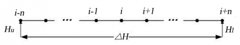
Suppose there are a total of (2n+1) discrete values of a formation parameter in the depth interval ΔH=[Hu, Hl] (Figure 2). Because the formation is continuous in space, the parameter must be similar and continuous within ΔH. Hence, the values of the formation parameter in ΔH can be treated as a measurement sample of the geological parameters at the depth of measuring pint i: {P(i-n), P(i-n+1), ..., P{i+n}}
Figure 2. Parameter sample
Considering the spatial variability of geological parameters, the sample interval should not be too large. Here, the interval is determined referring to the range of the variation function in the formation [12].
Let P(hk) be the values of geological parameter at the depths of hk(k=1, 2, ..., N) in the target stratum, and Δh be the depth interval. Then, the variation function can be established as:
$\gamma (\Delta h)=\frac{1}{2\left( N-1 \right)}\sum\limits_{k=1}^{N-1}{{{\left[ p({{h}_{k}})-p({{h}_{k}}+\Delta h) \right]}^{2}}}$ (3)
For each depth interval mΔh(m=1, 2, ..., N-1), the corresponding γ(mΔh) can be computed. Then, the corresponding theoretical variation function can be selected to fit the discrete points [mΔh, γ(mΔh)] (m=1, 2, ..., N-1). Once the theoretical model parameters are determined, the sample interval ΔH can be obtained as twice the range.
3.3 Probability distribution function
Let $\mu(\xi)$ be a Borel function on interval ΔH=[Hu, Hl] [18]. Then, the probability density of geological parameter at measuring point i can be estimated by:
${{\tilde{f}}_{i}}(p)=\frac{1}{(2n+1)C}\sum\limits_{i=1}^{2n+1}{\mu }\left( \frac{p-{{p}_{i}}}{C} \right)$ (4)
where, C is a positive and fixed window width.
According to theory of molecular diffusion [19], the explicit normal expression of the Borel function can be determined as:
$\mu (\xi )=\frac{1}{\sigma \sqrt{2\pi }}{{e}^{\frac{{{\xi }^{2}}}{2{{\sigma }^{2}}}}}$ (5)
Then, the probability density of the geological parameter normally dispersed in interval ΔH=[Hu, Hl] can be expressed as:
${{\tilde{f}}_{i}}(p)=\frac{1}{\sqrt{2\pi }(2n+1)h}\sum\limits_{j=i-n}^{i+n}{\left\{ \exp \left[ -\frac{{{\left( p-{{p}_{j}} \right)}^{2}}}{2{{h}^{2}}} \right] \right\}}$ (6)
where, $h=C \sigma$ is the dispersion coefficient.
Let pmax and pmin be geological parameter X in ΔH=[Hu, Hl], respectively. Then, the dispersion coefficient can be computed by:
$h=\frac{\lambda \left( {{p}_{\max }}-{{p}_{\min }} \right)}{2n}$ (7)
3.4 Formation matrix with credibility
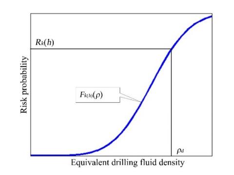
Since small probability events are not likely to occur, the cumulative probability function was interpolated with credibility (Figure 3), and the pressure values between upper and lower credibility limits were treated as the pressure matrix. In this way, the formation matrix with credibility can be obtained:
$\boldsymbol{M}_{B}^{\prime}=\left[\boldsymbol{H}, \boldsymbol{P}_{l}, \cdots, \boldsymbol{P}_{u}\right]=\left[\left[\begin{array}{c}h_{1} \\ \vdots \\ h_{i} \\ \vdots \\ h_{m}\end{array}\right]\left[\begin{array}{c}p_{l 1} \\ \vdots \\ p_{l i} \\ \vdots \\ p_{l m}\end{array}\right] \cdots\left[\begin{array}{c}p_{u 1} \\ \vdots \\ p_{u i} \\ \vdots \\ p_{u m}\end{array}\right]\right]$ (8)
Figure 3. Formation matrix with credibility
4.1 Hazard mechanism of drilling risks
In essence, drilling risk evaluation is to establish safety constraints for drilling, according to the influence of geological and engineering factors. Under static conditions, the pore pressure, collapse pressure, and facture pressure of the formation produce a safety density window for the drilling fluid, laying the basis for safe drilling design [4]. According to the actual drilling conditions, the boundary conditions of the safe density window are listed in Table 1.
Table 1. Boundary conditions of the safety density window for the drilling fluid
|
Type of safe drilling fluid |
Boundary conditions |
|
Lower limit of drilling fluid density to prevent well kick ρk(h) |
${{\rho }_{\text{k}}}(h)={{P}_{p}}(h)+{{S}_{\text{b}}}+\Delta \rho $. |
|
Lower limit of drilling fluid density to prevent wellbore collapse ρc(h) |
${{\rho }_{\text{c}}}(h)={{p}_{c}}(h)+{{S}_{\text{b}}}$ |
|
Upper limit of drilling fluid density to prevent differential pressure sticking ρsk(h) |
${{\rho }_{\text{sk}}}(h)={{P}_{p}}(h)+\frac{\Delta P}{h\times 0.0098}$ |
|
Upper limit of drilling fluid density to prevent lost circulation ρL(h) |
${{\rho }_{\text{L}}}(h)={{P}_{f}}(h)-{{S}_{\text{g}}}-{{S}_{\text{c}}}$ |
|
Upper limit of drilling fluid density to prevent lost circulation in well kill ρkl(h) |
${{\rho }_{\text{kl}}}(h)={{P}_{f}}(h)-{{S}_{\text{g}}}-{{S}_{\text{k}}}\times \frac{{{h}_{p\max }}}{h}$ |
For drilling safety, the density $\rho_{d}$ of drilling fluid during drilling, and the density $\rho_{kick}$ of drilling fluid to treat well kick should satisfy:
$\max \left\{ {{\rho }_{k}},{{\rho }_{cd}} \right\}\le {{\rho }_{d}}\le \min \left\{ {{\rho }_{L}},{{\rho }_{sk}},{{\rho }_{cu}} \right\}$
${{\rho }_{\text{kick}}}\le {{\rho }_{kl}}$ (9)
Judging by the safety density window, the following drilling risks will occur if the drilling fluid density fails to meet the above condition (Table 2).
Table 2. Types of drilling risks
|
Type of risk |
Hazard condition |
|
Well kick |
$\rho_{d}<\rho_{k}$ |
|
Wellbore collapse |
$\rho d<\rho c$ |
|
Lost circulation in well kill |
$\rho kick >\rho L$ |
|
Differential pressure sticking |
$\rho d>\rho_{s k}$ |
|
Lost circulation |
$\rho d>\rho L$ |
For the lack of space, well kick was cited as an example to explain how to calculate the probability of a drilling risk. The relationship between drilling fluid density and formation pressure is illustrated in Figure 4. In Figure 4(a), $\rho_{k}$ is the drilling fluid density to prevent well kick; In Figure 4(b), $\rho_{k}(j)$ is the drilling fluid density to prevent well kick at the cumulative probability of j, and $\rho_{d}$ is the drilling fluid density used for drilling.
For Figure 4(a), the formation pressure at depth h is a single value. If $\rho_{d}>\rho_{k}(h)$, the well kick will not occur; If $\rho_{d}<\rho_{k}(h)$, the well kick will occur.
For Figure 4(b), the lower limit of drilling fluid density $\rho_{k}(h)$ to prevent well kick at depth h is distributed in an interval, according to the concept of formation pressure matrix. If $\rho_{d}$ is greater than the upper limit of the interval $\rho_{k}\left(h, j_{\max }\right)$, the well kick will not occur; If $\rho_{d}$ is smaller than the lower limit of the interval $\rho_{k}\left(h, j_{\max }\right)$, the well kick will occur; if $\rho_{d}$ falls in the interval, the probability of well kick depends on the cumulative probability that $\rho_{k}(h)$ is greater than $\rho_{d}$.
After analyzing the hazard mechanism, formation pressure, and drilling fluid density, the calculation formulas of drilling risk probabilities (Table 3) were derived based on the GSSIT [20].
Table 3. Probabilities of drilling risks
|
Type of accident |
Risk probability |
|
Well kick |
Rk(h)=P(ρd>ρk(h))=1-Fρk(h)(ρd) |
|
Wellbore collapse |
Rc(h)=P(ρd>ρc(h))=1-Fρc(h)(ρd) |
|
Lost circulation |
Rsk(h)=P(ρd>ρsk(h))=Fρsk(h)(ρd) |
|
Differential pressure sticking |
RL(h)=P(ρd>ρL(h))=FρL(h)(ρd) |
|
Lost circulation in well kill |
RKL(h)=P(ρkick>ρL(h))=FρL(h)(ρkick) |
Note: Rk(h), Rc(h), Rsk(h), RL(h), and RkL(h) are the well kick risk, wellbore collapse risk, lost circulation risk, differential pressure sticking risk, and lost circulation risk in well kill; ρd is the density of the drilling fluid for drilling, g/cm3; ρkick is the annulus pressure gradient at the shut-in after well kick (expressed as equivalent drilling fluid density), g/cm3.
Risk probability can be calculated by probability theory or simulation. If the model is simple with a few stochastic variables, the distribution function of drilling risk probability could be directly derived from probability theory, and the risk probability could be determined by the distribution function. If the model is complex with many stochastic variables, theoretical analysis will be relatively difficult. In this case, the MC simulation [21, 22] can be introduced to easily compute the probability of each drilling risk. Hence, this paper selects MC simulation to determine the drilling risk probabilities.
(a) The formation pressure profile is a single curve.
(b) The formation pressure profile is a pressure distribution zone
Figure 4. Relationship between drilling fluid density and formation pressure
4.3 Evaluation steps
Taking well kick for example, the risk probability of a drilling risk can be evaluated as follows:
Step 1. Calculate the lower limit $\rho_{k}$ of drilling fluid density to prevent well kick.
The formation pressure matrix can be established according to the construction method for formation matrix with credibility:
${{P}_{p}}={{\left[ \begin{align} & p_{1{{j}_{\min }}}^{p}\cdots \ p_{1j}^{p}\cdots \ p_{1{{j}_{\max }}}^{p} \\ & \ \ \vdots \ \ \ \ \cdots \ \ \vdots \quad \cdots \ \ \vdots \\ & p_{i{{j}_{\min }}}^{p}\ \cdots \ p_{ij}^{p}\ \cdots \ p_{i{{j}_{\max }}}^{p} \\ & \ \vdots \ \ \ \ \ \cdots \ \ \vdots \quad \cdots \ \ \vdots \\ & p_{m{{j}_{\min }}}^{p}\cdots \ p_{mj}^{p}\cdots \ p_{m{{j}_{\max }}}^{p} \\ \end{align} \right]}_{m\times n}}$ (10)
For scientific calculation, it is necessary to establish a design coefficient matrix. If the coefficient has a single value, then the pumping pressure coefficient matrix and additional drilling fluid density matrix can be respectively expressed as:
${{S}_{b}}={{\left[ \begin{align} & a\cdots a\cdots a \\ & \ \vdots \ \cdots \ \vdots \ \ \cdots \vdots \\ & a\cdots a\cdots a \\ & \ \vdots \ \cdots \ \vdots \ \ \cdots \vdots \\ & a\cdots a\cdots a \\ \end{align} \right]}_{m\times n}}$,$\Delta \rho ={{\left[ \begin{align} & b\cdots b\cdots b \\ & \ \vdots \ \cdots \ \vdots \ \ \cdots \vdots \\ & b\cdots b\cdots b \\ & \ \vdots \ \cdots \ \vdots \ \ \cdots \vdots \\ & b\cdots b\cdots b \\ \end{align} \right]}_{m\times n}}$ (11)
Then, the lower limit of drilling fluid density to prevent well kick can be obtained as:
${{\rho }_{k}}={{P}_{p}}+{{S}_{b}}+\Delta \rho ={{(P_{ij}^{p}+a+b)}_{m\times n}}$ (12)
If the coefficient values are discrete or continuous, then the pumping pressure coefficient matrix and additional drilling fluid density matrix can be respectively expressed as:
${{S}_{b}}=\left[ \begin{align} & {{a}_{11}}\cdots {{a}_{1j}}\cdots {{a}_{1n}} \\ & \ \vdots \ \ \cdots \ \ \vdots \ \ \ \cdots \ \ \vdots \\ & {{a}_{i1}}\cdots {{a}_{ij}}\cdots {{a}_{in}} \\ & \ \vdots \ \ \cdots \ \ \vdots \ \ \ \cdots \ \ \vdots \\ & {{a}_{m1}}\cdots {{a}_{mj}}\cdots {{a}_{mn}} \\ \end{align} \right]$, $\Delta \rho =\left[ \begin{align} & {{b}_{11}}\cdots {{b}_{1j}}\cdots {{b}_{1n}} \\ & \ \vdots \ \ \cdots \ \ \vdots \ \ \ \cdots \ \ \vdots \\ & {{b}_{i1}}\cdots {{b}_{ij}}\cdots {{b}_{in}} \\ & \ \vdots \ \ \cdots \ \ \vdots \ \ \ \cdots \ \ \vdots \\ & {{b}_{m1}}\cdots {{b}_{mj}}\cdots {{b}_{mn}} \\ \end{align} \right]$ (13)
Then, the lower limit of drilling fluid density to prevent well kick can be obtained as:
${{\rho }_{k}}={{P}_{p}}+{{S}_{b}}+\Delta \rho ={{(P_{ij}^{p}+{{a}_{ij}}+{{b}_{ij}})}_{m\times n}}$ (14)
Figure 5. Probability of well kick
Step 2. Calculate the probability of well kick at depth h.
ρk(h) is the row vector at depth h. Through statistical analysis of ρk(h), the distribution function Fρk(h) at that depth can be obtained (Figure 5). Then, the probability of well kick at depth h can be derived as:
${{R}_{\text{k}}}(h)=P({{\rho }_{\text{d}}}<{{\rho }_{\text{k}}}(h))=1-{{F}_{{{\rho }_{\text{k}}}(h)}}({{\rho }_{\text{d}}})$ (15)
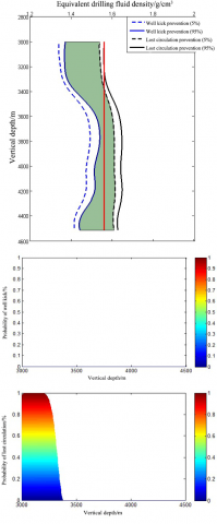
Well X is a key development well in Kekeya area of Tuha Basin. Multiple risks have occurred during the drilling. Historical data of the well show that: the outlet flow of drilling fluid increased at the depth of 3,900m, where the drilling fluid density was 1.5g/cm3. To prevent blowout, the drilling fluid density was adjusted to 1.56g/cm3. However, lost circulation occurred at 3,200m due to excessive pumping.
Considering the uncertainty of formation pressure, a formation pressure matrix was constructed, and used to evaluate the probabilities of drilling risks. Figures 6 and 7 present the evaluation results before and after the adjustment of drilling fluid density, respectively.
As shown in Figures 6 and 7, the drilling fluid density of 1.5g/cm3 was relatively low in the well section of 3,550-4,000m, owing to the high formation pore pressure. There was a high risk of well kick in this section. After the drilling fluid density was adjusted to 1.56g/cm3, there was a risk of lost circulation, for the new density is close to the fracture pressure of the formation. The evaluation results basically agree with the actual situation of the well.
Figure 6. Evaluation results at the drilling fluid density of 1.5g/cm3
Figure 7. Evaluation results at the drilling fluid density of 1.56g/cm3
(1) The proposed concept of formation matrix facilitates the collection, storage, management, analysis, and mapping of formation attributes, and accelerates the analysis, calculation, explicit expression and refresh of spatial operations.
(2) The formation matrix with credibility was established to scientifically describe formation parameters that contain certain errors. Based on the matrix, the drilling risk probabilities were evaluated based on the GSSIT and MC simulation. The proposed method was applied to evaluate the well kick risk of a well in Kekeya area of Tuha Basin. The evaluation results basically agree with the actual situation of the well, indicating that our method can effectively quantify drilling risks.
(3) The precision of formation matrix is the basis of drilling risk evaluation. If the matrix has a low credibility, the drilling risk evaluation will be very inaccurate, failing to provide a reference for the design of drilling plan. Theoretically, the formation matrix can illustrate the formation scientifically, only if sufficient information is fully utilized and fused. Then, it is possible to make reliable identification of drilling risks. Therefore, the future research will try to effectively fuse all kinds of drilling information, making them complement each other, and then establish a credible formation matrix and prepare a correct drilling plan.
The study was supported by the PetroChina Innovation Foundation (Grant. No.: 2017D-5007-0314).
[1] Aldred, W., Plumb, D., Bradford, I., Cook, J., Gholkar, V., Cousins, L., Minton, R., Fuller, J., Goraya, S., Tucker, D. (1999). Managing drilling risk. Oilfield Review, 11(2): 2-19. https://pdfs.semanticscholar.org/dffc/35a8a093e6b4fa1474456e82ef2f0e1c4038.pdf.
[2] Amir-Heidari, P., Maknoon, R., Taheri, B., Bazyari, M. (2016). Identification of strategies to reduce accidents and losses in drilling industry by comprehensive HSE risk assessment—a case study in Iranian drilling industry. Journal of Loss Prevention in the Process Industries, 44: 405-413. https://doi.org/10.1016/j.jlp.2016.09.015
[3] Abimbola, M., Khan, F., Khakzad, N., Butt, S. (2015). Safety and risk analysis of managed pressure drilling operation using Bayesian network. Safety Science, 76: 133-144. https://doi.org/10.1016/j.ssci.2015.01.010
[4] Mitchell, R.F., Miska, S.Z. (2011). Fundamentals of Drilling Engineering. Society of Petroleum Engineers.
[5] Phoon K.K. (2019). The story of statistics in geotechnical engineering. Georisk: Assessment and Management of Risk for Engineered Systems and Geohazards,14(1): 3-25. https://doi.org/10.1080/17499518.2019.1700423
[6] Deng, Z.P., Li, D.Q., Qi, X.H., Cao, Z.J., Phoon, K.K. (2017). Reliability evaluation of slope considering geological uncertainty and inherent variability of soil parameters. Computers and Geotechnics, 92: 121-131. https://doi.org/10.1016/j.compgeo.2017.07.020
[7] Cui, J., Jiang, Q., Li, S., Feng, X., Zhang, M., Yang, B. (2017). Estimation of the number of specimens required for acquiring reliable rock mechanical parameters in laboratory uniaxial compression tests. Engineering Geology, 222: 186-200. https://doi.org/10.1016/j.enggeo.2017.03.023
[8] Yasseri, S. (2017). Drilling risk identification, filtering, ranking and management. International Journal of Coastal and Offshore Engineering, 1(1): 17-26. http://ijcoe.org/article-1-27-en.html
[9] Khakzad, N., Khan, F., Amyotte, P. (2013). Quantitative risk analysis of offshore drilling operations: A Bayesian approach. Safety Science, 57: 108-117. https://doi.org/10.1016/j.ssci.2013.01.022
[10] Li, Q., Chang, D., Xu, Y., Tang, J., Liang, H. (2009). Drilling risk management system based on knowledge integration. Acta Pet Rolei Sinica, 30(5): 755-759.
[11] Wei K., Guan Z.C, Ma J.S., Qi, J.T., Sheng, Y.N. (2015). Assessment method for uncertainty of geological parameters in well drilling. Journal of China University of Petroleum, 39(5): 89-93. https://doi.org/10.3969/j.issn.1673-5005.2015.05.012
[12] Wei, K., Guan, Z.C., Wei, J.H., Fu, S.L., Zhao, T.F. (2013). Drilling engineering risk evaluation method based on neural network and Monte-Carlo simulation. Zhongguo Anquan Kexue Xuebao, 23(2): 123-128. https://doi.org/10.16265/j.cnki.issn1003-3033.2013.02.016
[13] Guan, Z.C., Wei, K., Fu, S., Zhao, T. (2013). Risk evaluation method for drilling engineering based on interval analysis. Petroleum Drilling Techniques, 41(4): 15-18. https://doi.org/10.3969/j.issn.1001-0890.2013.04.004
[14] Bhandari, J., Abbassi, R., Garaniya, V., Khan, F. (2015). Risk analysis of deepwater drilling operations using Bayesian network. Journal of Loss Prevention in the Process Industries, 38: 11-23. https://doi.org/10.1016/j.jlp.2015.08.004
[15] Charles, R., Ryzhikov, K. (2015). Merganser Field: managing subsurface uncertainty during the development of a salt diapir field in the UK Central North Sea. Geological Society, London, Special Publications, 403(1): 261-298. https://doi.org/10.1144/SP403.15
[16] Liang, H., Zou, J., Liang, W. (2019). An early intelligent diagnosis model for drilling overflow based on GA–BP algorithm. Cluster Computing, 22(5): 10649-10668. https://doi.org/10.1007/s10586-017-1152-5
[17] Reber, J.E., Cooke, M.L., Dooley, T.P. (2020). What model material to use? A Review on rock analogs for structural geology and tectonics. Earth-Science Reviews, 202: 103107. https://doi.org/10.1016/j.earscirev.2020.103107
[18] Juang, C.H., Zhang, J., Shen, M.F., Hu, J.Z. (2019). Probabilistic methods for unified treatment of geotechnical and geological uncertainties in a geotechnical analysis. Engineering Geology, 249: 148-161. https://doi.org/10.1016/j.enggeo.2018.12.010
[19] Hristopulos, D.T., Baxevani, A. (2020). Effective probability distribution approximation for the reconstruction of missing data. Stochastic Environmental Research and Risk Assessment, 1-15. https://doi.org/10.1007/s00477-020-01765-5
[20] Bhuyan, P., Dewanji, A. (2017). Estimation of reliability with cumulative stress and strength degradation. Statistics, 51(4): 766-781. https://doi.org/10.1080/02331888.2016.1277224
[21] Athens, N.D., Caers, J.K. (2019). A Monte Carlo-based framework for assessing the value of information and development risk in geothermal exploration. Applied Energy, 256: 113932. https://doi.org/10.1016/j.apenergy.2019.113932
[22] Moselhi, O., Roghabadi, M.A. (2020). Risk quantification using fuzzy-based Monte Carlo simulation. Journal of Information Technology in Construction (ITcon), 25(5): 87-98. https://doi.org/10.36680/j.itcon.2020.005