Andik Isdianto*![]() | Intan Astritya Anggraini
| Intan Astritya Anggraini![]() | Gilang Rusrita Aida
| Gilang Rusrita Aida![]() | Rhochmad Wahyu Illahi
| Rhochmad Wahyu Illahi![]() | Rudianto
| Rudianto![]() | Muhammad Naufal Eka Putra
| Muhammad Naufal Eka Putra![]() | Uun Yanuhar
| Uun Yanuhar![]() | Nico Rahman Caesar
| Nico Rahman Caesar![]() | Aulia Lanudia Fathah
| Aulia Lanudia Fathah![]() | Alifiulahtin Utaminingsih
| Alifiulahtin Utaminingsih![]() | Mohammad Maskan
| Mohammad Maskan![]() | Berlania Mahardika Putri
| Berlania Mahardika Putri![]() | Dwi Candra Pratiwi
| Dwi Candra Pratiwi
© 2025 The authors. This article is published by IIETA and is licensed under the CC BY 4.0 license (http://creativecommons.org/licenses/by/4.0/).
OPEN ACCESS
Cities need decision-ready tools to convert satellite heat evidence into enforceable planning rules in tropical coastal contexts. This study quantifies how land-cover composition shapes land surface temperature (LST) in North Jakarta’s Penjaringan District and translates findings into policy metrics. Methodology: We mapped land cover (Google Earth object-based image analysis) and retrieved LST from Landsat (2005–2024). Variables were aggregated on a 150 × 150 m grid (n = 242) and related via ordinary least squares to estimate class-specific effects. Results & Conclusions: Built-up area expanded (+113%) while mangroves increased (+77%); cool LST classes collapsed and warm classes proliferated. Regression yields a stable hierarchy: built-up is the strongest warming driver; mangroves provide the strongest natural cooling; water and other vegetation also cool. On a per-fraction basis, mangrove cooling effectiveness is ~59% of built-up warming. These results establish quantitative, planning-scale evidence that nature-based assets can materially blunt urban heating in a dense coastal setting. Implications: We operationalize the evidence into four auditable indicators—Minimum Green-Space per Block, Canopy Connectivity Index, Per-Parcel Pervious Ratio, and a Cooling-Deficit Limit—and an adaptation-zoning workflow targeting persistent hotspots, impervious corridors, and coastal buffers. The metrics fit routine permitting and support annual, satellite-based audits, offering a replicable path to climate-resilient urban development.
blue-green infrastructure, coastal megacity, land surface temperature, mangrove conservation, object-based image analysis, remote sensing for planning, urban heat mitigation, urban planning indicators
Tropical coastal megacities are experiencing rapid land conversion that reconfigures surface energy balances and intensifies surface urban heat, observable in land surface temperature (LST) patterns [1, 2]. For planners, the central question is not merely whether heat is rising, but which land-cover configurations most effectively moderate LST and how that evidence can be translated into enforceable planning instruments and monitoring routines [3, 4].
Jakarta exemplifies these dynamics. In the northern coastal Penjaringan District, large-scale development and reclamation have altered land–water interfaces over the past two decades amid documented regional warming signals [5]. Within this setting, mangrove ecosystems are strategic assets—buffering coasts [6], storing blue carbon [7], and sustaining biodiversity [8]—yet remain under urbanization pressure that can erode their climatic and ecological services [7, 8].
Advances in Earth observation now support planning-scale diagnostics of land cover and LST [9], enabling cities to relate spatial composition to thermal outcomes with consistency over time [10]. Nevertheless, in tropical coastal contexts, the literature rarely provides comparative, decision-ready estimates of cooling effectiveness across distinct land covers (e.g., mangroves, other vegetation, water bodies, ponds) [11] that planners can embed in zoning, development control, and investment prioritization [2, 3].
This study responds to that gap for Penjaringan (North Jakarta). Using high-resolution Google Earth imagery with Object-Based Image Analysis (OBIA) [12], and Landsat-based thermal retrievals [10], we quantify spatiotemporal LULC–LST relationships (2005–2024) and derive empirical coefficients that rank class-level cooling. Crucially, we translate these findings into a policy framework—adaptation priorities and auditable indicators aligned with SDG 11 (sustainable, resilient cities) and SDG 13 (climate action) [13]—to support integration of green–blue infrastructure (including mangroves) within statutory planning and routine performance monitoring [4].
Contributions. (i) An empirically grounded ranking of land-cover cooling effectiveness in a tropical coastal megacity; (ii) a planning-ready conversion of these results into indicators suitable for zoning and development control [4]; and (iii) an alignment pathway that connects satellite monitoring with SDG-oriented urban cooling policy and investment decisions [13].
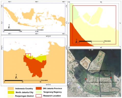
2.1 Study area
The study focuses on Penjaringan District (North Jakarta), a rapidly urbanizing coastal fringe comprising reclaimed islands, dense settlements, traditional aquaculture ponds, open water, and the Muara Angke–Kapuk mangrove system (Figure 1). The area typifies Southeast Asian megacity trade-offs where development pressure intersects with ecosystem conservation and climate adaptation needs.
Figure 1. Research area
2.2 Data source
We combined high-resolution optical imagery and thermal satellite data to quantify land cover and land surface temperature (LST) over time:
2.3 Pre-processing
All scenes underwent geometric/radiometric correction; atmospheric correction was applied as appropriate to ensure time-series consistency before LST retrieval and index computation [10]. ETM+ SLC-off artifacts were gap-filled using multi-date compositing to improve spatial continuity for analysis and visualization [10].
2.4 LST retrieval
We retrieved LST from ETM+ Band 6 and TIRS Band 10 using a standard single-channel workflow—radiance → brightness temperature → NDVI-based emissivity correction → LST (℃) [15]. Outputs were resampled to 30 m and harmonized across years for comparison at planning scales [10].
2.5 Land-cover mapping (OBIA)
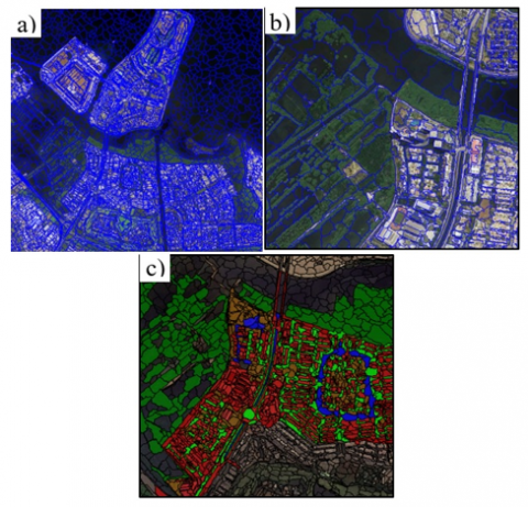
Land cover was mapped with Object-Based Image Analysis (OBIA) in eCognition, combining spectral, textural, and shape/context features [12]. Land cover classification was performed using eCognition Developer software (Figure 2). The initial stage involved image segmentation using the Multiresolution Segmentation algorithm with parameters scale = 50, shape = 0.5, and compactness = 0.5. This segmentation scale was chosen because the resulting segments were able to distinguish different land cover objects quite well. In the classification process, training samples were created from each land cover class. The segmented objects were then classified using the Nearest Neighbor Classification algorithm based on the average spectral value of each band and basic shape features. The OBIA methods used can vary because they are adjusted to the researcher's needs, such as the scale of the research area, level of detail, and others (Figure 3).
Figure 2. Land classification flow with OBIA in this study
Figure 3. Stages of OBIA: (a) Segmentation, (b) Detail of segment, (c) Classification
Six classes were delineated to align with planning-relevant decisions—Built-up, Mangrove, Water body, Pond, Open land, Non-mangrove vegetation—and temporal stacks (2005, 2010, 2015, 2020, 2024) supported change detection [9]. We define some of our land cover classes (Table 1).
Table 1. Definition of land cover types
|
Land Cover Types |
Definition |
|
Mangrove |
A type of tropical vegetation that grows along the coast or river estuaries, influenced by the ebb and flow of seawater, and has a muddy substrate. It has a dark green canopy and dense texture with a high vegetation spectrum. |
|
Built-Up Land |
Land covered by permanent or semi-permanent buildings so that rainwater does not fall directly onto the surface, visible in the form of settlements, public facilities, roads, industry, and others. |
|
Open Land |
Land that has very little or no vegetation cover or buildings, such as fields, initial clearing of agricultural land, former fires or logging, is brownish in color (open land, open fields, etc.). |
|
Water Body |
Natural and artificial waters that are permanent or semi-permanent, such as seas, rivers, reservoirs, wetland rice fields that contain water, and others. |
|
Pond |
Artificial aquaculture areas, generally located in coastal areas, consist of deliberately controlled pools of water designed to support aquatic organisms. They are characterized by geometrically shaped, compartmentalized, and unnatural pools of water. |
|
Non-Mangrove Vegetation |
Terrestrial vegetation other than mangroves includes urban trees, shrubs, and others. |
2.6 Spatial aggregation and indicators
To link Earth observation with planning units, we summarized all variables on a 150 m × 150 m grid (n = 242), computing (a) mean LST (℃) and (b) area of each land-cover class per cell to support block/neighborhood-scale diagnostics used by municipal planners [3, 4]. This study uses a spatial analysis unit in the form of a 150 m × 150 m grid for several reasons. First, the resolution of Landsat 8 imagery (30 m) allows one grid to contain 25 LST pixels, resulting in a more stable average value, in line with previous studies that applied smoothing using a 5 × 5 pixel window. Second, the grid size is a multiple of the original image resolution, making it consistent, easy to replicate, and suitable for LST-based spatial analysis. In addition, empirical studies show that the relationship between LST and urban morphology tends to be stable at a scale of ± 150 m, so this size is considered ideal for capturing local variability and analyzing the relationship between land cover and surface temperature.
In this study, land-cover maps derived from OBIA classification were overlaid with a 150 × 150 m grid. For each grid cell, the absolute area (in hectares) of each land-cover type—built-up, mangrove, water body, aquaculture pond, non-mangrove vegetation, and open land—was calculated. These area values were directly used as independent variables and statistically related to the mean LST of each grid cell, without converting them into proportional or fractional values.
2.7 Statistical analysis
We estimated ordinary least squares regressions with LST as the dependent variable and class fractions as predictors to quantify the influence of each land-cover type on LST [2, 16]:
$Y=a_0+a_1 \cdot X_1+a_2 \cdot X_2+\ldots+a_n \cdot X_n$ (1)
where, Y is the dependent variable (LST), X1, X2,...,Xn represent the independent variables (e.g., built-up area, vegetation, water bodies, ponds, other land cover types), and a0, a1,...,an are the regression coefficients [2, 16]. This analysis quantified the influence of each land cover type on LST, providing insight into how land conversion impacts local thermal conditions.
2.8 Translation to planning metrics
Rather than emphasizing raw magnitudes in the main text, we use the signs and relative ordering of coefficients to derive operational planning elements—(i) adaptation priorities (restorative greening; albedo–permeability management; coastal buffers) and (ii) auditable indicators (minimum green-space per block, canopy connectivity, per-parcel pervious ratio, neighborhood cooling-deficit limit)—that can be monitored from the same EO streams [1, 3, 4].
3.1 Land-cover dynamics in a coastal megacity fringe
3.1.1 Urban intensification and loss of evapotranspiring surfaces
Penjaringan’s coastal fringe reflects the typical trade-off of fast-growing tropical megacities: built-up area nearly doubled from 716.1 ha (2005) to 1,525.1 ha (2024; +113%) (Table 1; Figure 4). Over the same period, water bodies declined from 2,046.8 to 1,520.4 ha (–25.7%) and ponds from 520.6 to 194.6 ha (–62.6%) (Table 1; Figure 4). Annualised rates underscore the structural shift: built-up expanded by ~42.6 ha·yr⁻¹, while water bodies and ponds contracted by ~27.7 ha·yr⁻¹ and 17.2 ha·yr⁻¹, respectively, amounting to a net –852.4 ha reduction in aquatic/pond surfaces across two decades (Table 2). These conversions replace evapotranspiring, heat-buffering surfaces with impervious materials that absorb and store heat, a well-documented pathway for surface warming during urban expansion [17, 18].
Table 2 presents the area of each land cover class during the period 2005–2024, indicating changes in land use composition in the study area. To better understand the dynamics of change, Table 3 displays the total area change and annual rate of change (ha/year) of each land cover class between 2005 and 2024. This presentation allows analysis based not only on the magnitude of change, but also on the speed and direction of the trend of change.
Table 2. Area of land cover types in 2005-2024 at research sites
|
Land Cover |
Area (Ha) |
||||
|
2005 |
2010 |
2015 |
2020 |
2024 |
|
|
Built-up Area |
716.10 |
940.20 |
1,211.60 |
1,340.50 |
1,525.10 |
|
Mangrove |
183.70 |
230.00 |
247.20 |
283.50 |
324.60 |
|
Water Body |
2,046.80 |
2,054.80 |
1,474.90 |
1,606.50 |
1,520.40 |
|
Pond |
520.60 |
325.60 |
223.00 |
197.30 |
194.60 |
|
Open Land |
211.10 |
74.60 |
638.50 |
303.40 |
164.90 |
|
Non Mangrove Veg. |
570.00 |
623.20 |
453.00 |
517.10 |
518.80 |
Table 3. Annual rate of change (2005-2024)
|
Land Cover |
Area (Ha) |
Area Change (∆ Area) |
Annual Rate of Change (Ha/year) |
|
|
2005 |
2024 |
|||
|
Built-up Area |
716.10 |
940.20 |
+809.00 |
+42.58 |
|
Mangrove |
183.70 |
230.00 |
+140.90 |
+7.41 |
|
Water Body |
2,046.80 |
2,054.80 |
-526.40 |
-27.70 |
|
Pond |
520.60 |
325.60 |
-326.00 |
-17.16 |
|
Open Land |
211.10 |
74.60 |
-46.20 |
-2.43 |
|
Non Mangrove Veg. |
570.00 |
623.20 |
-51.20 |
-2.69 |
Functionally, the loss of open-water/pond area reduces latent-heat flux and heat capacity at block scale, weakening daytime evaporative cooling and dampening nocturnal heat release (Table 2) [18]. Conversely, enlarging built-up fractions raise sensible-heat flux, thermal storage, and radiative trapping in compact corridors/blocks with low permeability, pushing local LST baselines upward (Figure 4) [17]. For planning, these quantified shifts flag priority geographies for permeability upgrades and strategic retention of water/vegetation to blunt added warming from new impervious cover, keeping cooling services close to densifying tracts (Table 2; Figure 5) [18].
Figure 4. Land cover changes in 2005-2024 at the research site
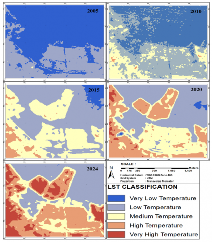
Figure 5. LST changes in 2005-2024 at the research site
We validated the OBIA maps against independent reference points visually interpreted from Google Earth Pro (~2 m) using stratified random sampling by class in each observation year (2005, 2010, 2015, 2020, 2024). We used a sample of 50 points per class for a total of 300 accuracy test points. Accuracy was summarised by overall accuracy (OA), Cohen’s κ, and per-class F1 (precision/recall). Table 4 provides the results of the accuracy test with kappa coefficients consisting of OA, Cohen's k, and per-class F1.
Table 4. Results of land cover classification accuracy tests
|
Year |
2005 |
2010 |
2015 |
2020 |
2025 |
|
OA |
83.06% |
90.46% |
87.67% |
88% |
93.69% |
|
Cohen’s k |
0.762394 |
0.865753 |
0.836733 |
0.835831 |
0.91265 |
|
Per-Class F1 |
|||||
|
Built-Up Land |
0.6977 |
0.9048 |
0.8862 |
0.8478 |
0.9565 |
|
Mangrove |
0.9286 |
0.9677 |
0.8485 |
0.8571 |
0.9674 |
|
Water |
0.9318 |
0.9395 |
0.9479 |
0.9264 |
0.9345 |
|
Pond |
0.5817 |
0.7797 |
0.8571 |
0.8800 |
0.9285 |
|
Open land |
0.7090 |
0.5600 |
0.7692 |
0.6977 |
0.7333 |
|
Non-Mangrove Vegetation |
0.9083 |
0.9535 |
0.8070 |
0.9459 |
0.9275 |
3.1.2 The mangrove “paradox”: resilience under pressure
Against this trend, mangrove cover expanded by ~77% (183.7 → 324.6 ha), an atypical yet policy-salient outcome for a dense coastal metropolis (Table 2; Figure 5). When protected and restored, mangroves function as multi-benefit infrastructure—buffering coasts, reducing wave energy and stabilising edges along urban shorelines [6], storing blue carbon with high long-term sequestration potential, supporting mitigation co-benefits [7], and sustaining local ecosystem services in Angke–Kapuk and similar urban mangrove mosaics, including recreation and water-quality functions [8]. The observed rebound is consistent with targeted restoration and shoreline management that preserve moisture availability and canopy structure, enabling latent-heat dominated cooling relative to adjacent built tracts (Table 2; Figure 5) [7].
3.1.3 Planning meaning: cooling demand and anchor assets for GBI
The land-cover shifts imply rising cooling demand in densifying blocks, where baseline LST increases necessitate stronger marginal cooling from each intervention (Table 2) [3]. In parallel, mangroves can be leveraged as anchor assets within green–blue infrastructure networks, providing edge-focused cooling that does not compete with inland development footprints (Figure 5) [13]. Aligning conservation/expansion with urban-form controls (albedo–permeability upgrades) and water-surface retention creates a coherent pathway to SDG-oriented climate resilience, linking diagnostics to zoning and permitting triggers (Table 2, Figure 5) [3].
3.1.4 Comparative context and likely mechanisms
Penjaringan’s trajectory mirrors coastal urbanisation patterns where conversion of evapotranspiring surfaces (water/ponds/vegetation) into impervious materials elevates heat storage and daytime LST, while fragmented green space limits advective/evaporative cooling [17]. Regional evidence further associates urban sprawl configurations with intensified SUHI signatures, reinforcing the temperature response to built-up expansion [19]. Within this context, the 77% mangrove expansion is policy-salient: protected/restored mangroves buffer coastal edges and supply cooling co-benefits without displacing inland development, making them prime candidates for edge-anchored GBI strategies (Table 2, Figure 5) [7]. Mechanistically, dense canopy, higher leaf-area index, and sustained moisture availability increase latent-heat exchange and reduce surface radiometric temperatures relative to built-up tracts, aligning observed cooling with vegetation physiology and surface-energy balance theory [18]. This biophysical logic supports an edge-focused conservation approach where urban form meets coastal systems, keeping cooling services proximate to heat-exposed neighbourhoods (Figure 5) [1].
3.2 Thermal transformation and loss of refugia
3.2.1 Warming signal and widening extremes
Multi-temporal LST analysis indicates a systematic warming across the period: the mean increased from 20.2℃ (2005) to 27.7℃ (2024) (+7.5℃), the minimum from 17.1℃ to 23.6℃ (+6.5℃), and the maximum from 27.0℃ to 36.0℃ (+9.0℃), widening the annual range from 9.9℃ to 12.4℃ (Table 5, Figure 6) [5, 20]. Most notably, “very low” LST zones contracted from ~84.7% of the landscape (3,593.1 ha of ~4,242 ha) to ~0.01% (0.3 ha), while “high/very high” zones expanded to ~49.3% by 2024 (2,092.9 ha) (Table 6), signaling a shift from refuge-rich mosaics toward more uniformly warm surfaces consistent with long-term warming signals and surface-UHI amplification in Jakarta and comparable cities [5, 20].
Table 5. LST value at the research site
|
Years |
LST Min (℃) |
LST Max (℃) |
LST Mean (℃) |
|
2005 |
17.10 |
27.00 |
20.20 |
|
2010 |
19.30 |
30.40 |
23.20 |
|
2015 |
21.80 |
30.40 |
24.90 |
|
2020 |
20.20 |
34.00 |
26.06 |
|
2024 |
23.60 |
36.00 |
27.70 |
Table 6. LST classification in 2005-2024 at the research site
|
LST Class |
Area (Ha) |
|
||||
|
2005 |
2010 |
2015 |
2020 |
2024 |
||
|
Very Low |
3,593.10 |
1,863.10 |
212.40 |
42.40 |
0.30 |
|
|
Low |
646.50 |
1,690.70 |
1,987.20 |
1,743.50 |
1,393.80 |
|
|
Medium |
2.40 |
676.80 |
1,816.40 |
1,234.30 |
754.90 |
|
|
High |
0.00 |
11.30 |
225.90 |
1,150.50 |
1,442.00 |
|
|
Very High |
0.00 |
0.00 |
0.00 |
71.10 |
650.90 |
|
3.2.2 Implications for passive cooling and ecosystem exposure
The contraction of low-temperature classes reduces neighborhood-scale passive-cooling options (shading and evapotranspiration from vegetation and open water) and raises exposure for heat-sensitive ecosystems (Table 6) [21]. In planning terms, the baseline has shifted upward: interventions must now deliver higher marginal cooling merely to restore prior thermal states before producing net improvements, which aligns with evidence that green–blue surfaces suppress LST while impervious expansion elevates it via increased sensible-heat flux and thermal storage [22].
3.2.3 Policy translation—decision-ready thresholds
To keep computation off the policy critical path, we express the analytics as auditable indicators derived from the same EO streams used here:
These thresholds are compatible with planning-scale monitoring and development-control workflows, enabling direct linkages from satellite-derived thermal evidence to zoning, permitting, and investment prioritisation.
3.2.4 Sensitivity of class thresholds and temporal context
Because Table 6 relies on thresholds, small shifts in class cut-offs or interannual anomalies can move marginal pixels across categories; therefore we emphasise multi-epoch persistence (e.g., remaining High/Very High in ≥ 2 of the last 3 epochs) over single-year status—the same logic embedded in the Restorative Priority rule—so planning targets structural heat patterns rather than year-specific noise (Tables 5-6, Figure 6) [1]. Cross-sensor Landsat time-series comparability and handling of ETM+ SLC-off artifacts are addressed in preprocessing to maintain trend reliability [10]. Where seasonal composites are available, applying the same classing to wet/dry seasons can refine intervention timing while preserving consistent indicators and audit thresholds [24].
3.3 Cooling effectiveness hierarchy (regression evidence)
3.3.1 Stable ordering of class effects
Grid-level OLS modelling at 150 × 150 m (n = 242) yields a consistent hierarchy of class-specific effects on LST (Table 7): Built-up exerts the strongest warming, while mangroves provide the strongest natural cooling, followed by water bodies, non-mangrove vegetation, and ponds (Table 7). Interpreted as ℃ per unit land-cover fraction within a grid cell, these coefficients are directly comparable across classes and thus decision-ready for planning arithmetic, aligning with broader evidence that surface composition governs thermal outcomes in cities [1, 2].
Model performance and basic diagnostics (reported here in full): overall R² = 0.951, all predictors significant at p < 0.001, residuals show no conspicuous trend against fitted values on visual inspection, and signs/magnitudes are consistent with physical expectations (warming for imperviousness; cooling for vegetated/blue classes) [1, 2].
Table 7 shows the influence of land-cover types on Land Surface Temperature (LST) using single-year data from 2024. The analysis was conducted on n = 242 grid cells (150 × 150 m) with complete land-cover and LST information. Table 5 was conducted using a single-year dataset (year 2024 only. The year 2024 was selected because the contrast in LST values among land-cover classes is most pronounced, allowing clearer interpretation of land-cover influence on LST. The sample size of n = 242 represents grid cells (150 × 150 m) with complete and consistent land-cover and LST data within the study area.
Table 7. Regression coefficients
|
Predictor (Fraction) |
Unstandarized Coefficients |
P-Value |
|
|
B |
Std. Error |
||
|
(Constant) |
28.086 |
0.94 |
<0.001 |
|
X1 (Built Area) |
1.619 |
0.69 |
<0.001 |
|
X2 (Mangrove) |
-0.960 |
0.95 |
<0.001 |
|
X3 (Open Land) |
1.139 |
0.69 |
<0.001 |
|
X4 (Water Body) |
-0.478 |
0.70 |
<0.001 |
|
X5 (Pond) |
-0.275 |
0.72 |
<0.001 |
|
X6 (Non Mangrove Vegetation) |
-0.469 |
0.59 |
<0.001 |
Notes: coefficients are interpreted at the analysis scale (150 m grid); signs/order are stable, supporting policy translation based on the hierarchy even when point magnitudes are kept lightweight in narrative
Multiple linear regression analysis (Table 7) shows that built-up and bare land variables have a significant positive effect on increasing land surface temperature (LST), while vegetation cover (mangrove and non-mangrove) and water bodies and ponds contribute to temperature reduction. These results confirm the differences in ecological function between land cover types, with built-up areas accelerating the warming process, while vegetation and water play a cooling role [25]. To strengthen these findings, a Pearson correlation analysis was also conducted (Table 8) which presents the direction and strength of the relationship between each variable and LST in a bivariate manner.
Table 8. Cross-sectional correlations between LST and land-cover fractions (2024)
|
Predictor (Fraction) |
Pearson (r) |
P-Value |
Direction |
|
X1 (Built Area) |
+0.829 |
<0.001 |
Warming |
|
X2 (Mangrove) |
-0.675 |
<0.001 |
Cooling |
|
X3 (Open Land) |
+0.495 |
<0.001 |
Warming |
|
X4 (Water Body) |
-0.737 |
<0.001 |
Cooling |
|
X5 (Pond) |
-0.558 |
<0.001 |
Cooling |
|
X6 (Non Mangrove Vegetation) |
-0.776 |
<0.001 |
Cooling |
The correlation results show a pattern consistent with the regression, where built-up land (r = +0.829; p < 0.001) and open land (r = +0.495; p < 0.001) are positively related to LST, while vegetation, water bodies, and ponds have a significant negative correlation (r ranging from –0.558 to –0.776; p < 0.001). Thus, the second table is presented as a complement to confirm the direction of the relationship that has been shown in the regression model, while also showing the magnitude of the cooling contribution of vegetation, especially mangroves, to temperature control in coastal areas [26].
This analysis reflects a simple bivariate relationship between each land cover type and LST without considering other variables. Meanwhile, the results of multiple linear regression provide a more complex picture because they simultaneously consider the contribution of each predictor variable. This confirms that although simple correlations between vegetation and water bodies have been shown to have a cooling effect, multiple regression shows that the contribution of this temperature reduction remains significant even after the influence of other variables is controlled [22]. The combination of these two analyses provides a more complete understanding that increasing built-up land exacerbates the phenomenon of surface warming, while vegetation, especially mangroves, plays a crucial role in maintaining the thermal balance of coastal areas.
This trend can be further clarified through a simple model showing the relationship between LST vs built-up land and LST vs mangroves in Figure 6.
Figure 6. Scatter plot LST vs built area
The regression analysis results show a positive relationship between LST values and built-up land area (y = 0.2392x – 6.0431; R² = 0.6013). This means that increases in built-up land area tend to be followed by increases in land surface temperature. The coefficient of determination (R²) value of 0.60 indicates that approximately 60% of the variation in LST can be explained by changes in built-up land area. This finding confirms that built-up areas contribute significantly to increasing surface temperatures, in line with the urban heat island phenomenon [27].
In contrast, the regression results between LST and mangrove area showed a negative relationship (y = –0.1913 × +5.9305; R² = 0.4555). This means that increasing mangrove area is associated with a decrease in land surface temperature. The R² value of 0.45 indicates that approximately 45% of the variation in LST can be explained by mangrove area. This finding supports the role of mangrove ecosystems as natural coolers capable of lowering surface temperatures through shading and evapotranspiration [28]. Overall, these two findings show that land cover changes in coastal areas have significant implications for surface temperature dynamics, where the dominance of built-up land increases the risk of warming, while the presence of mangroves serves as an important mitigating factor.
3.3.2 Magnitude for planning arithmetic (kept lightweight)
For scenario testing, multiply each coefficient by the proposed change in class fraction and sum the terms to estimate the net block-scale ΔLST [1, 2]. On a per-fraction basis, mangrove cooling ≈ 59% of built-up warming (|β_mangrove| / β_built-up ≈ 0.960/1.619 ≈ 0.59), indicating substantial offset potential where conservation/restoration is feasible (Table 7). The value ‘≈59% cooling effectiveness’ refers only to the per-unit-area effect (−0.960/1.619) derived from the regression coefficients. However, in absolute terms, built-up areas cover 1,525.1 ha, while mangroves cover only 324.6 ha. When multiplying the coefficients by actual area (area-weighted impact), total cooling by mangroves amounts to −311.6℃/ha, which is only about 12.6% of the total warming effect from built-up areas (2,468.3℃/ha). Then the value ‘59%’ refers to the cooling potential per unit area, not the total contribution at the landscape scale. This accords with the role of mangroves as multi-benefit green–blue infrastructure in coastal cities [29].
3.3.3 How we use the hierarchy
To avoid over-emphasising point estimates, we use the signs and ordering to guide siting (where to intervene first) and sizing (how much of each class to target), while the full coefficients and basic diagnostics are provided above for transparency (Table 7). This directly enables planning tools such as restorative greening in built-dominated cells, coastal buffers anchored by mangroves, and permeability/albedo upgrades in persistent warm corridors, within standard development-control workflows [30, 31].
3.3.4 Worked example: block-scale ΔLST arithmetic
A redevelopment adds +0.10 built-up in a 150 × 150 m block but restores +0.02 mangrove and +0.03 water. Using Table 5:
$\begin{array}{r}\Delta L S T \approx(1.619 \times 0.10)-(0.960 \times 0.02) -(0.478 \times 0.03) =+0.128^{\circ} \mathrm{C}(\text { approx. })\end{array}$
Two takeaways: (i) modest green–blue additions can materially blunt added warming, and (ii) the relative ordering is often sufficient for siting/sizing decisions, while exact coefficients remain available for audit and replication [1, 2, 7].
3.3.5 Robustness and limits (for prudent use)
Three boundary conditions matter in planning deployment: (i) coefficients are average effects at 150 m; micro-site morphology and roughness/height can cause local departures [17, 18]; (ii) effects reflect the observed composition envelope of Penjaringan—extreme scenarios outside this envelope merit caution [1, 2]; (iii) directional stability (signs/order) across epochs underpins policy use even when precise magnitudes are de-emphasised in the text [1, 2].
3.4 Design and planning translation
Evidence above is translated into three implementation channels that connect thermal diagnostics with development control and investment decisions.
3.4.1 Targeting principles
Restorative greening is directed to blocks that persist as hotspots—cells remaining in High/Very High LST classes in ≥ 2 of the last 3 epochs—and also exhibit low existing green share, so added evapotranspiration capacity is placed where thermal stress is chronically highest (Figure 6; Table 6). This targeting reflects the well-established pattern that transitions toward built surfaces elevate LST by replacing moisture-available, vegetated or water surfaces with impervious materials that suppress latent-heat flux (Table 2; Figure 5) [32].
In parallel, albedo–permeability upgrades are prioritised along compact impervious corridors and large blocks, where material properties and limited infiltration jointly amplify sensible-heat storage; minimum pervious-surface ratios and higher-reflectance finishes can therefore be enforced at the permitting stage (Table 2; Figure 5) [33, 34].
Along the coastal edge, buffers that protect and, where feasible, expand mangroves at built-up margins act as anchor assets within the green–blue network, leveraging thermal moderation [35], coastal protection [6], and blue-carbon storage [7] (Figure 4). Taken together, these targeting rules convert the LULC–LST diagnostics into place-specific actions that concentrate cooling where deficits are largest, upgrade materials where heat accumulates, and secure edge-based nature-based solutions under coastal urbanisation pressures.
3.4.2 Auditable indicators
To embed thermal outcomes in routine planning, four indicators can be updated annually from the same EO streams used here. First, a Minimum green-space per block (%) prioritised where block LST exceeds a neighbourhood threshold derived from the Table 3 class distributions links directly to evidence that greener blocks exhibit lower LST via shading and evapotranspiration [36], and that expanding green share in built-dominated tracts yields measurable surface-cooling dividends [35]. Table 9 is the threshold recommendation for the first indicator.
Table 9. Recommended threshold range for the first indicator
|
Indicator |
Operational Definition |
Formula Method |
Recommended Threshold |
|
Minimum Green Open Space per Block |
Percentage of vegetated surface within one urban block or analysis grid |
%Green = (Vegetated Area/Total Block Area) × 100 |
Minimum : ≥ 20% (Optimal : ≥ 30%) |
Table 10. Recommended threshold range for the second indicator
|
Indicator |
Operational Definition |
Formula Method |
Recommended Threshold |
|
Canopy Connectivity Index |
Degree of spatial connectivity between vegetated patches within the landscape |
Connectivity = Patch Cohesion Index or Connectance Index |
≥ 0.50 |
LST regression shows cooling effect emerges when vegetation exceeds 20% of a block and 30% aligns with Indonesian National Spatial Planning Regulation (PP No. 26/2007) and urban climate studies. Second, a Canopy Connectivity Index measuring functional links among parks, street trees, and riparian strips within a set distance supports advective/evaporative cooling by sustaining continuous vegetated corridors, consistent with findings that more connected green space moderates the urban thermal environment across seasons [37], and acts as a thermal regulator at district scale [38]. Table 10 is the threshold recommendation for the second indicator.
Values above 0.5 indicate functional ecological connectivity and effective cooling continuity and supported by landscape ecology literature. Third, a Per-parcel Pervious Ratio (minimum share of pervious/vegetated surfaces enforced at permitting) addresses the material and hydrologic controls on heat storage and sensible-heat flux, reflecting multi-city results that higher imperviousness elevates LST while greener/pervious configurations suppress it [39], with metropolitan evidence from Kuala Lumpur reinforcing the sensitivity of LST to built–green surface composition in permitting-scale decisions [40]. Table 11 is the threshold recommendation for the third indicator.
Table 11. Recommended threshold range for the third indicator
|
Indicator |
Operational Definition |
Formula Method |
Recommended Threshold |
|
Per-Parcel Pervious Ratio |
Minimum proportion of pervious or vegetated surfaces that must be maintained within each land parcel or development lot as part of the building permitting process |
Pervious Ratio (%) = (Pervious or vegetated area / total parcel area) × 100 |
Minimum : ≥ 20% (Preferred : ≥ 30%) |
High imperviousness increases land surface temperature (LST) and sensible heat flux. Empirical studies show LST rises with built-up density and decreases with pervious/green surfaces. A minimum of 20–30% aligns with cooling thresholds and international planning practices. Fourth, a Cooling-Deficit Limit (Δ ℃)—the allowable deviation of block-level LST from the district seasonal baseline—provides a trigger for stronger greening/permeability requirements once exceeded, aligning with planning-scale LULC–LST diagnostics that translate satellite thermal evidence into development control thresholds [41], and with regression-based planning applications that use EO-derived indicators for zoning and approvals [42]. Collectively, these indicators anchor zoning conditions and investment prioritisation in observed LULC–LST relationships at decision scales, enabling auditable, annually updatable benchmarks for urban cooling policy [43]. Table 12 is the threshold recommendation for the fourth indicator.
Table 12. Recommended threshold range for the fourth indicator
|
Indicator |
Operational Definition |
Formula Method |
Recommended Threshold |
|
Cooling Deficit Threshold (∆℃) |
Temperature gap between actual LST and expected LST under optimal vegetation conditions |
∆ = LST Actual – LST Predicted Ideal |
∆ ≥ 1.5℃ indicates cooling deficit |
This threshold is based on regression coefficients which built up area increases LST by +1.619℃ per ha, while mangrove cools -0.960℃/ha, then a 1.5℃ gap reflects insufficient ecosystem cooling.
3.4.3 Scenario arithmetic
Net thermal change at block or neighbourhood scale can be estimated directly from the regression by combining proposed class-fraction deltas with their coefficients (ΔLST ≈ Σ βᵢΔXᵢ), allowing planners to test alternatives without bespoke modelling each cycle [1, 2].
Warming from added built-up fraction can be counterbalanced by conserving or restoring mangroves, water, and other vegetation according to the observed hierarchy in Table 5. For illustration, adding +0.10 built-up while restoring +0.02 mangrove and +0.03 water gives: ΔLST ≈ (1.619 × 0.10) − (0.960 × 0.02) − (0.478 × 0.03) = +0.128℃ (approx.), showing how modest green–blue additions can materially blunt added warming at block scale (Table 7).
Two caveats guide prudent use: coefficients represent average effects at 150 m, so micro-site morphology and material choices (albedo/permeability) can cause local departures and should be addressed through corridor upgrades [17, 18]; and reliable estimates are obtained when scenarios remain within the composition envelope observed in Penjaringan’s record, keeping results traceable to documented local responses [1, 2].
3.4.4 Implementation sequencing and governance hooks
We adopt a two-step sequence aligned with routine planning cycles. Target & condition. Apply the Cooling-Deficit Limit together with a persistence rule (cells remaining in High/Very High classes in ≥ 2 of the last 3 epochs) to shortlist restorative blocks/corridors, and—along the coastal edge—prioritise mangrove frontages where local drivers of change and anthropogenic pressures (e.g., clearing decisions) have historically governed gains and losses in canopy and extent (Table 6; Figure 5) [44].
For shortlisted areas, embed Per-parcel Pervious Ratios and Minimum green-space per block in permits to reduce sensible-heat storage and raise evapotranspiration, while consolidating mangrove buffers as climate-adaptation infrastructure where built margins meet tidal waters (Figure 5) [45, 46]. These controls complement evidence that strategically vegetated/pervious parcels deliver distributed infiltration and runoff-delay benefits at district scale, strengthening thermal and hydrologic performance in compact fabrics [47]. Delivery should be co-produced with local stewardship groups and community organisations that have demonstrated effectiveness in Indonesia’s coastal cities, improving compliance, maintenance, and ecological outcomes for mangrove projects [48-50]. Where municipalities repurpose vacant or under-used land, pairing regeneration with green-infrastructure economics enhances feasibility and long-term operations and maintenance [51].
3.5 Policy and planning implications
The LST–land cover relationships derived here translate into operational planning metrics at decision scales using the 150 × 150 m grid summaries and the class coefficients in Table 5 to target and size cooling actions by block or corridor [1, 2]. In practice, the coefficients serve as prioritisation indicators: expand green corridors and riparian strips where built fractions dominate and advective/evaporative exchange is limited (Table 2; Figure 5) [51]; protect and restore mangroves as edge-anchored green–blue infrastructure delivering strong cooling with co-benefits (Tables 2, 7; Figure 5) [52]; and increase surface permeability/albedo in compact fabrics to curb sensible-heat storage (Tables 2, 7) [53]. Given the observed ordering of effects, these signals can be converted into area-based cooling targets at block or neighbourhood scale—i.e., required ΔX in built, mangrove, vegetation, and water—anchored to the model’s ℃-per-fraction coefficients (Table 7) [54, 55].
A zoning translation follows from the hotspot analysis (Table 6; Figure 6). (i) Restorative zones: persistently warm blocks (High/Very High in ≥ 2 of the last 3 epochs) advance to greening to expand canopy and improve connectivity within the urban fabric [18]. (ii) Albedo–permeability management zones: dense built-up areas adopt minimum pervious-surface shares and higher-reflectance finishes at permitting to reduce storage and raise latent flux [17]. (iii) Coastal/semi-coastal buffer zones: shore-adjacent tracts secure and, where feasible, expand mangrove belts as multi-benefit thermal and resilience infrastructure at the built edge [56].
These metrics can be embedded in statutory instruments (e.g., RDTR/RTRK, zoning ordinances) as auditable indicators tied to observed LST: a minimum green-space per block, canopy-connectivity thresholds, a per-parcel pervious-surface ratio, and a Cooling-Deficit Limit that caps block-level LST deviation from the district seasonal baseline (Tables 5-6; Table 5) [57]. Targets can be set with the study’s arithmetic—e.g., where a block exceeds the baseline, the required mix of ΔX (mangrove/vegetation/water vs. built) is sized so that ΣβᵢΔXᵢ ≤ 0 at the 150 m scale, keeping calculations traceable to local coefficients (Table 7) [1].
Because the indicators are remotely monitorable, annual compliance and progress checks can be run from the same Earth-observation streams used here—harmonised Landsat LST time series and global mangrove/urban mapping—to maintain methodological continuity across years [58, 59]. Coupling these audits with routine plan reviews enables mid-course corrections (e.g., tightening pervious-ratio thresholds where High-class persistence remains, or redirecting restorative greening to new hotspots) and provides an evidence base for reallocating budgets toward the best thermal returns [60, 61]. This science-to-policy pipeline supports explicit trade-off analysis (e.g., add green space vs. reduce impervious cover) and supplies the technical justification for investments that yield thermal and public-health co-benefits at city scale [3, 4].
The framework advances SDG 11 by improving spatial quality and equitable access to green space—conditions repeatedly associated with cooler urban surfaces [62]—and operationalises SDG 13 by mainstreaming climate adaptation into land-use planning through measurable, spatially explicit indicators [63, 64]. In coastal settings, securing and restoring mangroves aligns development with low-carbon, climate-resilient pathways via blue-carbon storage and multifunctional ecosystem services at the urban shoreline.
This study demonstrates that land‐cover change in the Penjaringan coastal fringe has materially reconfigured the surface thermal regime and that these dynamics can be translated into auditable, decision‐scale planning metrics. Built-up area nearly doubled between 2005 and 2024 (+113%), while water bodies (–25.7%) and ponds (–62.6%) contracted; in contrast, mangroves expanded by ~77% (Table 2; Figure 5). Over the same period, LST means and extremes rose (mean: 20.2℃ → 27.7℃), with “very low” LST classes collapsing from ~84.7% of the landscape to ~0.01% and “high/very high” classes reaching ~49.3% by 2024 (Tables 5--6; Figure 6). Grid-level regression at 150 m (n = 242) achieved strong fit (R² = 0.951) and a stable hierarchy of effects: built-up warms most (+1.619℃ per unit fraction), while mangroves cool most among natural classes (–0.960), followed by water (–0.478), non-mangrove vegetation (–0.469), with open land warming (+1.139) (Table 7). On a per-fraction basis, mangrove cooling is ~59% of built-up warming, providing clear arithmetic for offsetting scenarios at block/neighbourhood scales (Table 7).
These results are policy-relevant in three ways. First, they convert satellite diagnostics into targeting rules—restorative greening for persistent hotspots with low green share, albedo–permeability upgrades in compact impervious corridors, and coastal buffers that secure/expand mangroves at built margins—so cooling is concentrated where deficits are largest. Second, they define four annually updatable indicators that link zoning and permitting to measurable outcomes: minimum green-space per block, canopy connectivity, per-parcel pervious ratio, and a Cooling-Deficit Limit referenced to the district’s seasonal LST baseline. Third, they provide lightweight scenario arithmetic (ΔLST ≈ Σ βᵢΔXᵢ) that keeps computation off the policy critical path while retaining traceability to locally estimated coefficients (Table 7).
Two limitations should guide interpretation. Effects are estimated as averages at 150 m and may not capture micro-site departures driven by 3D form, material albedo, or roughness; and the indicators rely on thresholded LST classes, so multi-epoch persistence (≥ 2 of the last 3 epochs) is preferred over single-year status to minimise sensitivity to marginal class shifts (Tables 5-6). The coefficients are most reliable within the observed composition envelope of Penjaringan; extrapolation to extreme, unobserved mixes warrants caution (Table 7).
Future work that remains consistent with the evidence presented here includes: seasonal stratification of the same indicators to refine intervention timing; explicit incorporation of 3D morphological and material variables alongside class fractions; operational calibration of the Cooling-Deficit Limit to local baselines; and continued annual EO audits using harmonised time series to evaluate whether upgraded corridors exit persistent high-LST classes and whether restorative blocks recover low-temperature classes (Tables 5-6; Figures 5-6). Overall, the study offers a replicable, audit-ready pathway for embedding LST–land-cover relationships into statutory planning and routine monitoring to advance urban cooling and climate resilience at decision scales.
The authors would like to thank all parties who have contributed to the completion of this research. This article is the result of an independent study and received no specific funding from any agency in the public, commercial, or not-for-profit sectors.
[1] Patel, S., Indraganti, M., Jawarneh, R.N. (2024). A comprehensive systematic review: Impact of land use/ land cover (LULC) on land surface temperatures (LST) and outdoor thermal comfort. Building and Environment, 249: 111130. https://doi.org/10.1016/j.buildenv.2023.111130
[2] Tran, D.X., Pla, F., Latorre-Carmona, P., Myint, S.W., Caetano, M., Kieu, H.V. (2017). Characterizing the relationship between land use land cover change and land surface temperature. ISPRS Journal of Photogrammetry and Remote Sensing, 124: 119-132. https://doi.org/10.1016/j.isprsjprs.2017.01.001
[3] Hasyim, A.W., Sukojo, B.M., Anggraini, I.A., Fatahillah, E.R., Isdianto, A. (2025). Urban heat island effect and sustainable planning: Analysis of land surface temperature and vegetation in Malang City. International Journal of Sustainable Development and Planning, 20(2): 683-697. https://doi.org/10.18280/ijsdp.200218
[4] Hasyim, A.W., Sukojo, B.M., Fatahillah, E.R., Anggraini, I.A., Isdianto, A. (2025). Assessing the impact of population density and land use on land surface temperature for sustainable urban planning in Malang City, Indonesia. International Journal of Sustainable Development and Planning, 20(5): 1679-2197. https://doi.org/10.18280/ijsdp.200533
[5] Siswanto, S., van Oldenborgh, G.J., van der Schrier, G., Jilderda, R., van den Hurk, B. (2015). Temperature, extreme precipitation, and diurnal rainfall changes in the urbanized Jakarta city during the past 130 years. International Journal of Climatology, 36(9): 3207-3225. https://doi.org/10.1002/joc.4548
[6] Shu, A., Zhu, J., Cui, B., Wang, L., Zhang, Z., Pi, C. (2023). Coastal wave-energy attenuation by artificial wooden fences deployed for mangrove restoration: An experimental study. Frontiers in Marine Science, 10. https://doi.org/10.3389/fmars.2023.1165048
[7] Alongi, D.M., Murdiyarso, D., Fourqurean, J.W., Kauffman, J.B., Hutahaean, A., Crooks, S., Lovelock, C.E., Howard, J., Herr, D., Fortes, M., Pidgeon, E., Wagey, T. (2015). Indonesia's blue carbon: A globally significant and vulnerable sink for seagrass and mangrove carbon. Wetlands Ecology and Management, 24(1): 3-13. https://doi.org/10.1007/s11273-015-9446-y
[8] Sumarga, E., Sholihah, A., Srigati, F.A.E., Nabila, S., Azzahra, P.R., Rabbani, N.P. (2023). Quantification of ecosystem services from urban mangrove forest: A case study in Angke Kapuk Jakarta. Forests, 14(9): 1796. https://doi.org/10.3390/f14091796
[9] Giri, C. (2021). Recent advancement in mangrove forests mapping and monitoring of the world using earth observation satellite data. Remote Sensing, 13(4): 563. https://doi.org/10.3390/rs13040563
[10] Holden, C.E., Woodcock, C.E. (2016). An analysis of Landsat 7 and Landsat 8 underflight data and the implications for time series investigations. Remote Sensing of Environment, 185: 16-36. https://doi.org/10.1016/j.rse.2016.02.052
[11] Mas'uddin, M., Karlinasari, L., Pertiwi, S., Erizal, E. (2023). Urban heat island index change detection based on land surface temperature, normalized difference vegetation index, and normalized difference built-up index: A case study. Journal of Ecological Engineering, 24(11): 91-107. https://doi.org/10.12911/22998993/171371
[12] Gu, H., Li, H., Yan, L., Liu, Z., Blaschke, T., Soergel, U. (2017). An object-based semantic classification method for high resolution remote sensing imagery using ontology. Remote Sensing, 9(4): 329. https://doi.org/10.3390/rs9040329
[13] Jaramillo, F., Desormeaux, A., Hedlund, J., Jawitz, J., et al. (2019). Priorities and interactions of sustainable development goals (SDGs) with focus on wetlands. Water, 11(3): 619. https://doi.org/10.3390/w11030619
[14] Madarasinghe, S.K., Yapa, K.K.A.S., Jayatissa, L.P. (2020). Google Earth imagery coupled with on-screen digitization for urban land use mapping: Case study of Hambantota, Sri Lanka. Journal of the National Science Foundation of Sri Lanka, 48(4): 357. https://doi.org/10.4038/jnsfsr.v48i4.9795
[15] Kumar, D., Shekhar, S. (2015). Statistical analysis of land surface temperature--vegetation indexes relationship through thermal remote sensing. Ecotoxicology and Environmental Safety, 121: 39-44. https://doi.org/10.1016/j.ecoenv.2015.07.004
[16] Basri, H. (2019). Pemodelan regresi berganda untuk data dalam studi kecerdasan emosional. Didaktika: Jurnal Kependidikan, 12(2): 103-116. https://doi.org/10.30863/didaktika.v12i2.179
[17] Cai, H., Xu, X. (2017). Impacts of built-up area expansion in 2D and 3D on regional surface temperature. Sustainability, 9(10): 1862. https://doi.org/10.3390/su9101862
[18] Yang, C., He, X., Wang, R., Yan, F., Yu, L., Bu, K., Yang, J., Chang, L., Zhang, S. (2017). The effect of urban green spaces on the urban thermal environment and its seasonal variations. Forests, 8(5): 153. https://doi.org/10.3390/f8050153
[19] Carneiro, E., Lopes, W., Espindola, G. (2021). Linking urban sprawl and surface urban heat island in the Teresina--Timon conurbation area in Brazil. Land, 10(5): 516. https://doi.org/10.3390/land10050516
[20] Ayanlade, A., Aigbiremolen, M.I., Oladosu, O.R. (2021). Variations in urban land surface temperature intensity over four cities in different ecological zones. Scientific Reports, 11: 20537. https://doi.org/10.1038/s41598-021-99693-z
[21] Arjasakusuma, S., Yamaguchi, Y., Hirano, Y., Zhou, X. (2018). ENSO- and rainfall-sensitive vegetation regions in Indonesia as identified from multi-sensor remote sensing data. ISPRS International Journal of Geo-Information, 7(3): 103. https://doi.org/10.3390/ijgi7030103
[22] Isdianto, A., Hasyim, A.W., Sukojo, B.M., Alimuddin, I., Anggraini, I.A., Fatahillah, E.R. (2025). Integrating urban design with natural dynamics: Enhancing ecological resilience in Malang City over a decade. International Journal of Sustainable Development and Planning, 20(3): 1061-1075. https://doi.org/10.18280/ijsdp.200313
[23] Maulana, J., Bioresita, F. (2023). Monitoring of land surface temperature in Surabaya, Indonesia from 2013-2021 using Landsat-8 imagery and Google Earth Engine. IOP Conference Series: Earth and Environmental Science, 1127(1): 012027. https://doi.org/10.1088/1755-1315/1127/1/012027
[24] Govil, H., Guha, S., Dey, A., Gill, N. (2019). Seasonal evaluation of downscaled land surface temperature: A case study in a humid tropical city. Heliyon, 5(6): e01923. https://doi.org/10.1016/j.heliyon.2019.e01923
[25] Hasyim, A.W., Anggraini, I.A., Usman, F., Isdianto, A. (2025). Evaluating urban heat island effects in Malang City parks using UAV and OBIA technologies. International Journal of Sustainable Development and Planning, 20(4): 1633-1644. https://doi.org/10.18280/ijsdp.200425
[26] Sumarmi, S., Purwanto, P., Bachri, S. (2021). Spatial analysis of mangrove forest management to reduce air temperature and CO2 emissions. Sustainability, 13(14): 8090. https://doi.org/10.3390/su13148090
[27] Saini, R., Rawat, S., Semwal, P., Singh, S., Chaudhary, S.S., Jaware, T.H., Patel, K.K. (2024). Improving built-up extraction using spectral indices and machine learning on Sentinel-2 satellite data in Mumbai suburban district, India. Traitement du Signal, 41(3): 1609-1623. https://doi.org/10.18280/ts.410348
[28] Hsieh, H.L., Lin, H.J., Shih, S.S., Chen, C.P. (2015). Ecosystem functions connecting contributions from ecosystem services to human wellbeing in a mangrove system in northern Taiwan. International Journal of Environmental Research and Public Health, 12(6): 6542-6560. https://doi.org/10.3390/ijerph120606542
[29] Narayan, S., Beck, M.W., Reguero, B.G., Losada, I.J., van Wesenbeeck, B., Pontee, N., Sanchirico, J.N., Ingram, J.C., Lange, G.M., Burks-Copes, K.A. (2016). The effectiveness, costs and coastal protection benefits of natural and nature-based defences. PLoS ONE, 11(5): e0154735. https://doi.org/10.1371/journal.pone.0154735
[30] Surjono, S., Fatahillah, E.R., Hasyim, A.W., Anggraeni, M., Jasmine, A.P., Isdianto, A. (2025). Urban harmony: Integrating spatial suitability and socio-economic factors to enhance quality of life in Kotalama riverbank settlements, Malang City, Indonesia. International Journal of Sustainable Development and Planning, 20(5): 1813-1829. https://doi.org/10.18280/ijsdp.200502
[31] Stipanović, V.B., Čukanović, J., Orlović, S., Atanasovska, J.R., Andonovski, V., Simovski, B. (2022). Linear greenery in urban areas and green corridors case study: Blvd. Bosnia and Herzegovina and Blvd. Hristijan Todorovski Karposh, Skopje, North Macedonia. Contemporary Agriculture, 71(3-4): 212-221. https://doi.org/10.2478/contagri-2022-0028
[32] Li, D., Sun, T., Liu, M., Yang, L., Wang, L., Gao, Z. (2015). Contrasting responses of urban and rural surface energy budgets to heat waves explain synergies between urban heat islands and heat waves. Environmental Research Letters, 10(5): 054009. https://doi.org/10.1088/1748-9326/10/5/054009
[33] Rossi, G., Iacomussi, P., Zinzi, M. (2018). Lighting implications of urban mitigation strategies through cool pavements: Energy savings and visual comfort. Climate, 6(2): 26. https://doi.org/10.3390/cli6020026
[34] Kappou, S., Souliotis, M., Papaefthimiou, S., Panaras, G., Paravantis, J.A., Michalena, E., Hills, J.M., Vouros, A.P., Ntymenou, A., Mihalakakou, G. (2022). Cool pavements: State of the art and new technologies. Sustainability, 14(9): 5159. https://doi.org/10.3390/su14095159
[35] Cordeiro, A., Ornelas, A., Lameiras, J.M. (2023). The thermal regulator role of urban green spaces: The case of Coimbra (Portugal). Forests, 14(12): 2351. https://doi.org/10.3390/f14122351
[36] Ziter, C.D., Pedersen, E.J., Kucharik, C.J., Turner, M.G. (2019). Scale-dependent interactions between tree canopy cover and impervious surfaces reduce daytime urban heat during summer. Proceedings of the National Academy of Sciences, 116(15): 7575-7580. https://doi.org/10.1073/pnas.1817561116
[37] Ornelas, A., Cordeiro, A., Lameiras, J.M. (2023). Thermal comfort assessment in urban green spaces: Contribution of thermography to the study of thermal variation between tree canopies and air temperature. Land, 12(8): 1568. https://doi.org/10.3390/land12081568
[38] Sun, F., Zhang, J., Yang, R., Liu, S., Ma, J., Lin, X., Su, D., Liu, K., Cui, J. (2023). Study on microclimate and thermal comfort in small urban green spaces in Tokyo, Japan---A case study of Chuo Ward. Sustainability, 15(24): 16555. https://doi.org/10.3390/su152416555
[39] Isa, N.A., Wan Mohd, W.M.N., Salleh, S.A. (2017). The effects of built-up and green areas on the land surface temperature of the Kuala Lumpur city. The International Archives of the Photogrammetry, Remote Sensing and Spatial Information Sciences, XLII-4/W5: 107-112. https://doi.org/10.5194/isprs-archives-xlii-4-w5-107-2017
[40] Hua, A.K., Ping, O.W. (2018). The influence of land-use/land-cover changes on land surface temperature: A case study of Kuala Lumpur metropolitan city. European Journal of Remote Sensing, 51(1): 1049-1069. https://doi.org/10.1080/22797254.2018.1542976
[41] Andries, A., Morse, S., Murphy, R., Lynch, J., Woolliams, E. (2019). Seeing sustainability from space: Using earth observation data to populate the UN Sustainable Development Goal indicators. Sustainability, 11(18): 5062. https://doi.org/10.3390/su11185062
[42] Hasyim, A.W., Ari, I.R.D., Kurniawan, E.B., Kriswati, L., Wahid, M.N.I., Isdianto, A. (2024). Integrating object-based classification and multivariate analysis to evaluate flood vulnerability in unplanned settlements of Malang City, Indonesia. International Journal of Design & Nature and Ecodynamics, 19(5): 1611-1625. https://doi.org/10.18280/ijdne.190515
[43] Zhao, H., Tan, J., Ren, Z., Wang, Z. (2020). Spatiotemporal characteristics of urban surface temperature and its relationship with landscape metrics and vegetation cover in rapid urbanization region. Complexity, 2020: 1-12. https://doi.org/10.1155/2020/7892362
[44] Maina, J.M., Bosire, J.O., Kairo, J.G., Bandeira, S.O., Mangora, M.M., Macamo, C., Ralison, H., Majambo, G. (2021). Identifying global and local drivers of change in mangrove cover and the implications for management. Global Ecology and Biogeography, 30(10): 2057-2069. https://doi.org/10.1111/geb.13368
[45] Arfan, A., Side, S., Nyompa, S., Maru, R., Sukri, I., Juanda, M.F. (2023). Structure and composition of mangrove vegetation in the Lakkang Delta and Lantebung, Makassar City, South Sulawesi, Indonesia. Forum Geografic, XXII(2): 151-158. https://doi.org/10.5775/fg.2023.2.3579
[46] Henri, H., Syafa'ati, R., Randiansyah, R. (2022). Species composition and vegetation structure of mangrove forest in Baskara Bakti Village, Central Bangka Regency, Bangka Belitung. IOP Conference Series: Earth and Environmental Science, 1108(1): 012004. https://doi.org/10.1088/1755-1315/1108/1/012004
[47] Kelleher, C., Golden, H.E., Burkholder, S., Shuster, W. (2020). Urban vacant lands impart hydrological benefits across city landscapes. Nature Communications, 11(1). https://doi.org/10.1038/s41467-020-15376-9
[48] Kurniawan, R.R., Suharini, E., Banowati, E. (2022). Mangrove conservation group management in Semarang City, Central Java, Indonesia. In Advances in Social Science, Education and Humanities Research. Atlantis Press. https://doi.org/10.2991/assehr.k.211125.085
[49] Majesty, K.I., Fadmastuti, M. (2018). Degree of community participation in mangrove resources management as livelihood support in West Java, Indonesia. E3S Web of Conferences, 74: 10005. https://doi.org/10.1051/e3sconf/20187410005
[50] Permana, S., Harefa, M.S., Tuhono, E., Rahmadi, M.T., Lubis, D.P., Restu, R., Novira, N., Sintong, M., Ginting, M.R.P., Halim, J., Habib, M. (2024). Community participation in mangrove conservation: The evidence from Blang Sebel, Simeulue. IOP Conference Series: Earth and Environmental Science, 1406(1): 012012. https://doi.org/10.1088/1755-1315/1406/1/012012
[51] Newman, G., Li, D., Zhu, R., Ren, D. (2018). Resilience through regeneration: The economics of repurposing vacant land with green infrastructure. Landscape Architecture Frontiers, 6(6): 10. https://doi.org/10.15302/j-laf-20180602
[52] Adulkongkaew, T., Satapanajaru, T., Charoenhirunyingyos, S., Singhirunnusorn, W. (2020). Effect of land cover composition and building configuration on land surface temperature in an urban-sprawl city, case study in Bangkok Metropolitan Area, Thailand. Heliyon, 6(8): e04485. https://doi.org/10.1016/j.heliyon.2020.e04485
[53] Helal, A., Zawawi, Z. (2024). Land cover and land surface temperature in the West Bank, Palestine. Advances in Civil Engineering, 2024(1). https://doi.org/10.1155/2024/1107242
[54] Abdulmana, S., Lim, A., Wongsai, S., Wongsai, N. (2021). Effect of land cover change and elevation on decadal trend of land surface temperature: A linear model with sum contrast analysis. Research Square. https://doi.org/10.21203/rs.3.rs-603120/v1
[55] Aflaki, A., Mirnezhad, M., Ghaffarianhoseini, A., Ghaffarianhoseini, A., Omrany, H., Wang, Z.H., Akbari, H. (2017). Urban heat island mitigation strategies: A state-of-the-art review on Kuala Lumpur, Singapore and Hong Kong. Cities, 62: 131-145. https://doi.org/10.1016/j.cities.2016.09.003
[56] Liu, W., Zhao, H., Sun, S., Xu, X., Huang, T., Zhu, J. (2022). Green space cooling effect and contribution to mitigate heat island effect of surrounding communities in Beijing Metropolitan Area. Frontiers in Public Health, 10. https://doi.org/10.3389/fpubh.2022.870403
[57] Rudianto, R., Darmawan, V., Isdianto, A., Bintoro, G. (2022). Restoration of coastal ecosystems as an approach to the integrated mangrove ecosystem management and mitigation and adaptation to climate changes in north coast of East Java. Journal of Coastal Conservation, 26: 37. https://doi.org/10.1007/s11852-022-00865-4
[58] García-Haro, A., Arellano, B., Roca, J. (2023). Quantifying the influence of design and location on the cool island effect of the urban parks of Barcelona. Journal of Applied Remote Sensing, 17(3): 034512. https://doi.org/10.1117/1.jrs.17.034512
[59] Bunting, P., Rosenqvist, A., Hilarides, L., Lucas, R.M., Thomas, N., Tadono, T., Worthington, T.A., Spalding, M., Murray, N.J., Rebelo, L.M. (2022). Global mangrove extent change 1996-2020: Global Mangrove Watch Version 3.0. Remote Sensing, 14(15): 3657. https://doi.org/10.3390/rs14153657
[60] Worthington, T.A., zu Ermgassen, P.S.E., Friess, D.A., Krauss, K.W., Lovelock, C.E., Thorley, J., Tingey, R., Woodroffe, C.D., Bunting, P., Cormier, N., Lagomasino, D., Lucas, R., Murray, N.J., Sutherland, W.J., Spalding, M. (2020). A global biophysical typology of mangroves and its relevance for ecosystem structure and deforestation. Scientific Reports, 10: 14652. https://doi.org/10.1038/s41598-020-71194-5
[61] Wang, Y., Lu, X., Wang, R., Jia, Y., Huang, J. (2023). Identification of bird habitat restoration priorities in a central area of a megacity. Forests, 14(8): 1689. https://doi.org/10.3390/f14081689
[62] Abougendia, S.M., Ayad, H.M., El-Sayad, Z.T. (2020). Classification framework of local climate zones using world urban database and access portal tools: Case study of Alexandria City, Egypt. In WIT Transactions on Ecology and the Environment. WIT Press, pp. 309-322. https://doi.org/10.2495/sdp200251
[63] Wang, Y., Guan, C. (2024). Integrating green space measures into future town planning in Zhejiang, China. Environment and Planning B: Urban Analytics and City Science, 52(4): 913-930. https://doi.org/10.1177/23998083241274913
[64] Stessens, P., Canters, F., Huysmans, M., Khan, A.Z. (2020). Urban green space qualities: An integrated approach towards GIS-based assessment reflecting user perception. Land Use Policy, 91: 104319. https://doi.org/10.1016/j.landusepol.2019.104319