Coastal Reef and Seagrass Monitoring for Coastal Ecosystem Management

In Indonesia, specific data on seagrass beds and coral reefs are fundamental in carrying out coastal ecosystem management. Seagrass beds and coral reefs are natural resources that provide enormous ecological benefits and contribute substantially to the sustainability of fishery resources in the country. These ecosystems actively produce nutrients for fish, entrap sediments, dissipate current and wave energy, recycle nutrients, and create a highly suitable habitat for shallow marine organisms [1, 2]. Similar to mangroves, they are known to absorb carbon dioxide (CO₂). According to the Indonesian Institute of Sciences, seagrass beds in Indonesia (293,464 ha) can sequester up to 1.9 to 5.8 megatons of CO₂ per year [3]. Also, coral reefs have a very promising yield of fishery products [4, 5].

Persistently growing human activities in coastal areas and the effects of climate change have led to the increased dynamics of seagrass cover. For instance, in Indonesia, these dynamics are indicated by changes in the seagrass cover conditions, from 46% coverage in 2015 to 37.58% in 2016, which continued to decrease until 2019 [6]. The Decree of the Indonesian Minister of Environment No. 200 of 2004 differentiates seagrass conditions into three categories based on percent cover of seagrasses in the region, namely healthy (with coverage above 60%), less healthy (30-59%), and unhealthy (<30%) [7]. Another decree issued by the same Minister, that is, No. 4 of 2001, divides the conditions of coral reefs into two classes, namely damaged (with coverage of 0-49%) and healthy (50-100%) [8]. The latest record shows that the seagrasses in the country cover 37.58% [3] and, therefore, fall into the category of unhealthy. Meanwhile, the percent cover of coral reefs is around 67% [6], signifying a healthy condition. Nevertheless, these states do not rule out the possibility of an annual decline. As confirmed by Waycott et al. [2] and Zhang [9], such changes do not only occur in Indonesia, but up to 29% of the seagrass bed and coral reef ecosystems worldwide have disappeared.

Seagrass bed and coral reef ecosystems need to continue to offer ecological, economic, and educational benefits for the community. Therefore, developing and updating coastal management measures are imperative as an attempt to preserve the conditions of these ecosystems. An example of an effective and efficient management tool is spatial analysis and multitemporal monitoring, which can be justified scientifically and used as a basis for managing seagrass bed and coral reef ecosystems sustainably. Both spatial analysis and multitemporal monitoring can utilize remote sensing technology to provide data for identifying and analyzing the dynamics of seagrass cover and the condition of coral reefs in specific locations. Remote sensing data can be used for spatial analysis at various scales and periodically, so it greatly facilitates multitemporal coastal monitoring. Remote sensing enables straightforward estimates and analyses of coastal marine ecosystems that change periodically. Also, it assists in the identification and evaluation of seagrass bed and coral reef ecosystem management that can contribute to the growth and preservation of coastal marine environments.

To be more efficient, this data is formed as a mapping model by utilizing the development of digital automation in the form of machine learning algorithms that are able to maximize the results of spatial analysis. This research adapts remote sensing technology for spatial and multitemporal analysis and machine learning algorithms. Especially as an initial stage to meet the information needs of coastal resources, especially coral reefs and seagrass beds, which can then be used for further analysis. This leads to the possibility of developing more universal mapping algorithm using satellite image for rapid mapping and monitoring of coral reef and seagrass [10]. Therefore, this research is expected to be used as a reference in similar studies, especially by government and stakeholders, when applying remote sensing data for coastal monitoring for coastal resources information for management purposes.

Because of its high effectiveness and efficiency, remote sensing has been widely used in coastal resource analysis [11-13]. Besides, with multitemporal remote sensing applications, patterns of changes over a particular range of years can be identified [14]. Remote sensing data have been used in several studies of seagrass bed and coral reef cover analysis and confirmed to produce excellent results [15-17]. Some examples of previous research [18] are mapped the biophysical characteristics of seagrass in the form of species, percent cover, and biomass in Moreton Bay using a variety of multispectral and airborne hyperspectral imagery. Lyons et al. [13] mapped percent of seagrass cover multi-temporal in Eastern Banks, Moreton Bay, Australia using OBIA. Roelfsema et al. [19] conducted a coral hierarchical mapping of coral reefs with different information scales. The hierarchy consists of reef, reef type, geomorphic zone and benthic community using object-based classification (OBIA) using IKONOS (4 m) and Quickbird (2.4 m) imagery. Roelfsema et al. [20] conducted a multi-temporal mapping of seagrass cover, species and biomass in Moreton Bay using a semi-automated object-based image analysis approach and had accurate results. Joyce and Phinn [21] developing spectral index for mapping live coral cover using multispectral and hyperspectral imagery integrated with a coral spectral library, and performing Spectral transformation, Water depth optical modeling, and Derivative analysis. Eastwood et al. [22] application of global protocols for quantitative coral reef health monitoring by considering the influence of increased tourism activities by utilizing Google Earth as a technology to accommodate reef check survey points. Wicaksono et al. [10] applied machine learning and cross validation approaches for mapping benthic habitats with high accuracy results. Previous research has shown that mapping coastal resources is very important for the sustainability of regional development and environmental management.

This research took place in Gili Sumber Kima, Buleleng Regency, Bali. This small island has potential seagrass bed and coral reef ecosystems and, at the same time, a somewhat massive development of tourism activities. There have been no inventories of seagrass beds and coral reefs around Gili Sumber Kima to date, and consequently, management activities are less than optimal. In response to this, the study sought to analyze changes in seagrass cover and damages to the coral reef in Gili Sumber Kima using a multitemporal approach and Sentinel 2A-MSI imagery. This multitemporal analysis is expected to be able to identify the spatial or temporal patterns of change in seagrass cover over a specific period and pinpoint the contributing factors. The research implications include the production of data on seagrass bed and coral reef ecosystems (inventory) that can be used as the basis for monitoring and managing coastal ecosystems.

3.1 Benthic habitat mapping

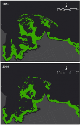
The benthic habitats were mapped using the major classes proposed by the Indonesian National Standard (SNI) and the technical guidelines for benthic habitat mapping issued by the data managers of P2O LIPI. Here, the major classes are substrate, coral reef, macroalgae, and seagrass. Benthic habitat maps were created by the multispectral classification of images that went through sunglint and water column corrections using the RF and SVM algorithms. The maps processed from images in two different years present different distributions and areas (Figure 3). From 2015 until 2019, the benthic habitats were experiencing some changes in their distributions and areas. The most noticeable change was the substrate. In 2015, the substrate cover was significantly wider than in 2019. This area reduction is believed to be the effect of climate, wave energy, current, and highly dynamic coastal waters [43, 44]. The same case applies to seagrass and coral reef covers. However, there was a misclassification in 2015 because the reflection of the coral reef was very similar to that of seagrass. Also, in 2019, the area of macroalgae had decreased, although not significantly.

Each classification result had different values of accuracy. RF algorithm with water column-corrected images as the channel input produced a classification of the 2019 data with the highest accuracy, 68.3%, and a kappa value of 52.89%. Meanwhile, in 2015, the highest accuracy (62.94%, with a kappa value of 42.25%) was produced by the SVM algorithm with sunglint-corrected images as the channel input (Table 2). The difference in accuracy was caused by the validation data that were sourced from 2019, meaning that when they were applied to the 2015 data, many validation points were either mismatched or non-existent. There was a high possibility that one point showed a benthic object in 2015 but a different one in 2019. As a result, the accuracy of the classification model in 2015 was lower than in 2019. This study is limited by the absence of temporal validation data for the year 2015. It assumed that the 2019 data could represent the appearance of benthic objects in 2015, as evidenced by the insignificant difference between the accuracies of the 2015 and 2019 classifications, i.e., 5-6%. The results of the experiment on benthic habitat classification are presented in Table 2.

Judging from the producer and user accuracies (Figure 4), seagrass cover from the best benthic habitat map in each year can be classified at high accuracy. In 2015, the map of the seagrass cover, which was produced using the SVM algorithm and sunglint-corrected images, had an accuracy of +-70%. Meanwhile, in 2019, through the RF algorithm and water column-corrected images, the mapped seagrass cover had an accuracy of +-83%. These figures demonstrate the ability of Sentinel-2A MSI as a data source that can classify marine objects correctly.

3-1.jpg

Figure 3. Benthic habitat map

Table 2. Benthic habitat map accuracy result

Based on the overall results of benthic habitat maps, DII bands have the lowest accuracy result. The benthic mapping concept emphasizes the variation aspects of pixel values on each object so the model can run optimally. Thus, when the pixel variation is very low, the model will saturate and cause a large error. In the DII band, the image pixel shows the object index value. Because each benthic object has similar DII values to another (low pixel variation). Thus, when the model is applied, saturation occurs, which produces high error in the maps. Another thing that affects the low accuracy of the 2015 benthic habitat map is the decreases of image quality when water column correction (DII) is applied (technical factors). The use of Sentinel-2 MSI images in very good clarity conditions, there is no need for additional correction or transformation treatments such as DII because it can worsen the pixel value of the image and decrease the accuracy [45].

4.png

Figure 4. Seagrass producer's (PA) and user's accuracy (UA) map

Using a machine-learning algorithm, it is very possible to include various datasets as classification inputs, in order to obtain an accurate benthic habitat map. Thus, the machine-learning algorithm may produce a classification result at the maximum image descriptive resolution. Regarding the machine learning classification algorithm, variations in the function parameters of both SVM and RF do not have a significant difference in results. This can be proven through a similar study using RF and SVM. [46] conducted an RF experiment for mapping seagrass beds. The scenarios used are five number of trees scenario, 25, 50, 75, 100, and 500. In addition, functions features, i.e., Square root of all features and Log of all features, and impurity in a node, i.e., Gini coefficient and Entropy. Based on the RF experiments, the results obtained are not very significant, its only differed 0.8 to 5.8% of the overall accuracy. This indicates that RF is a more consistent machine learning classification algorithm.

For the SVM algorithm, if the image quality is in very good condition, the results obtained will not have significant accuracy with RF. Both after applying kernel variations and the number of folds used. What is found in this research is that SVM is very sensitive with poor image quality (high noise). Therefore, the results obtained have lower accuracy than RF. However, RF provided more consistent performance in terms of spatial distribution and its similarity to the field condition compared with SVM [10]. As a suggestion for further research, especially machine learning algorithms so that they can be widely used. It is very important to pay attention to the band used. For instance, the quality of the corrected image of the water column is very subjective and depends on the condition of each area's waters. When the conditions are not favorable, the resulting model tends to give less good results. So that the best input band to use is Surface reflectance and deglint bands.

3.2 Seagrass change detection

Change detection helps to identify changes in seagrass cover from 2015 until 2019. This analysis can straightforwardly pinpoint the direction of the observed changes. Figure 4 shows that the estimated seagrass cover had an accuracy of +-70% in 2015 and +-83% in 2019. The classifications of seagrass cover had different accuracies because of many factors. From the data source, the contributing factors may include resolution, correction, data quality, and algorithm. The circumstances in the field may also be a factor, such as water clarity, seagrass depth, seagrass density, and sand substrate in the background.

In clear shallow waters, the sand substrate can simplify the identification process and improve the accuracy of the seagrass cover classification [13]. Sand and seagrass in clear shallow waters have contrasting reflections. The former has a light expression, while the latter is dark. With these characteristics, the seagrass and sand objects in the study area can be distinguished; therefore, the classified seagrass cover had high accuracy. Figure 5 shows the different distribution patterns of seagrass cover in 2015 and 2019. In the middle of the study area close to the sandbar, a significant difference was detected. In 2015, this point was a sand substrate, but in 2019, it had transformed into seagrass. The seagrass cover decreased from 243.3 ha in 2015 (including misclassification) to 185.2 ha in 2019. This decline illustrates significant changes in seagrass cover.

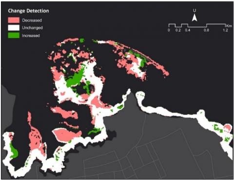
The change detection analysis produced three directions of change, namely decreasing, increasing, and unchanging (Figure 6). In the case of seagrass, the area of coverage was decreased by 86 ha and increased by 27.9 ha, whereas no sign of changes was found in the other 157 ha. The unchanging state represents seagrass habitats with preserved conditions that are protected from coastal processes and dynamics. However, the total loss of the seagrass area (changed into sand substrates) was approximately three times greater than the increase. Unless mitigated soon, this situation will negatively affect marine ecosystems. In 2015, the spatial distribution of the seagrass cover was better than in 2019. These changes are attributable to the hydrodynamic effects of waves and currents, as well as the influence of human activities. Cage culture and many other aquaculture practices, excessive exploitation of shellfish (clams), and blast fishing [47, 48] significantly affect the growth and development of seagrass cover in shallow waters. In the study area, many fish ponds have been built close to seagrass beds and coral reefs, and their number continues to grow. In the long term, this form of aquaculture brings about damages to seagrass cover, coral reefs, and fish habitats and deteriorates the quality of the waters. The interviews with the local community revealed that clam exploitation by bombs and crowbars were the leading cause of the damages in Gili Sumber Kima. According to the fishers, the perceived environmental damages included loss of fish and other marine organisms. This adversity reduced the total fishery products and threatened the continuity of fisher livelihoods. If this issue continues in the future, it will cause severe negative impacts on shallow-water habitats, especially seagrass cover.

5.png

Figure 5. Seagrass cover map of 2015 and 2019

6.jpg

Figure 6. Seagrass change detection map

Changes in seagrass cover are also attributable to climatic factors (wind, waves, strong currents) [15]. When severe weather occurs, it causes direct physical damage to the seagrass cover as it stirs up the sediments and mixes them with the chemical waste from the residential and lodging areas. In this case, seagrass cover cannot grow optimally. According to [2, 48], there is a positive correlation between the extent of land-use conversion to built-up environments and the significance of the seagrass cover shrinkage. In the future, to avoid the emergence of negative impacts, the condition of the waters and benthic habitats needs to be preserved so as to allow seagrass beds to grow and develop optimally. A sustainably healthy ecosystem is believed to bring a variety of rare aquatic organisms, such as turtles and dugongs that highly depend on seagrass as their source of food. Provided that any human activities that worsen the condition of these environments are significantly reduced, the existence of these sea creatures can stabilize the marine environments. Another positive impact of a healthy ecosystem is that coral reefs can improve their state of health and natural functions as fish habitats. In the future, similar research is expected to be able to develop or utilize data on ecosystems and shallow-water biodiversity to observe the development trend or pattern periodically [13].

3.3 Coral condition mapping

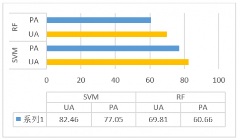
The maps of coral reef cover created in this study have high accuracy. The SVM and RF algorithms produced the accuracies of 77-80% and 60-70%, respectively (Figure 7). These percentages indicate that 60-80% of the estimated seagrass cover is closely similar to the actual condition in the field. The area of cover produced by the SVM algorithm has high accuracy and shows a similar distribution to the actual condition. Therefore, it was used as the boundary in the analysis of coral reef condition.

7.png

Figure 7. Graphic of Coral Reef Condistion Class Producer’s (PA) and User’s Accuracy (UA)

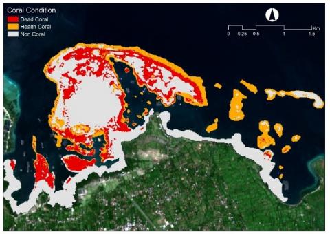
Based on the classification scheme, the mapping was carried out using two classes of coral reefs, namely damaged and healthy coral reefs. Either class was decided by comparing the percent of live coral reef cover with the dead one. If the percent of live coral reef cover is greater than the dead one, the object is classified as healthy. On the contrary, if the percent of dead coral reef cover is higher than the live one, the object falls into the category of damaged. The coral reef conditions were mapped using Sentinel-2 MSI images, whose level of correction already includes surface reflectance. At this level, the pixel value of the image can represent different coral reef conditions in the field, and in that year, the primary data were collected in the field. The results of the water column correction on Sentinel-2 MSI images were not used in the mapping because this correction would change the value of the image into the depth invariant index. The depth invariant index is not suitable for the mapping of coral reef conditions because it is significant in different types of objects. For instance, the damaged and healthy coral reefs in water column-corrected images have similar index values. Therefore, discriminating between the two states of health would be difficult. Meanwhile, using surface reflectance imagery, the conditions of coral reefs can be distinguished easily because the reflections correspond to the actual conditions of the objects in the field. Using a rather strong water column correction can cause damages or severe noises on the image and lead to a complex identification process and reduced accuracy [45].

The map of the coral reef conditions showed a fairly unique distribution. The damaged coral reefs were located in shallow waters, whereas the healthy ones were in deep waters (Figure 9). With 42% accuracy and a kappa value of 0.38, this map had a relatively low precision. This result is caused by the lack of sample size that causes some points to be misclassified during the calculation of the accuracy. Besides this is due to the similarity of pixels between coral reefs with different percent cover. The different depths also affected the value of the coral reef pixels. The deeper the coral reef, the lower the pixel reflectance and identified as a high coral live cover, and vice versa. The coral percent cover mapping results have accuracy and other problems that are comparable to those found in some studies [21]. Until now, coral percent cover mapping has rarely been attempted due to the low accuracy of the results. Based on the distribution pattern, the estimated state of the coral reefs resembled the actual condition—i.e., the damaged reefs were found in shallow waters but the healthy ones were in deep waters. A total of 1397 ha of coral reefs were damaged, while the healthy ones covered an area of 1505 ha (Table 3). In other words, almost 50% of the coral reefs around the waters of Gili Sumber Kima are damaged.

Table 3. Area of coral cover condition

8.png

Figure 8. Coral condition: a) Healthy coral; b) Dead coral

source: Field data (2019)

Massive human activities in coastal areas are known to cause damages to coral reefs. Humans affect their surroundings through the rapidly growing tourism activities, land-use conversion to settlements and tourism services, aquaculture, marine traffics, construction of infrastructure, and destructive fishing [49, 50]. The distribution of the damaged coral reefs in the shallow waters (Figure 8) seems to associate with the floating net cages, which cover a relatively large area close to the coral reefs. The intensive activities in this form of aquaculture affect the surrounding aquatic environments, leading to stressed and eventually damaged coral reefs. Also, most floating net cages are anchored or tied to coral reefs to prevent them from drifting. Aside from this cage culture, damages to coral reefs are induced by clam overexploitation and severe weather. Coral reefs are home to kima or giant clams that are protected and have high economic values. Around the waters of Gili Sumber Kima, these clams are harvested massively by damaging the coral reefs using crowbars. Consequently, many coral reefs are damaged in the process, especially in the north.

9.jpg

Figure 9. Coral condition map

Severe weather that hits the northern coast of Bali has caused many changes in the coastal region. Gili Sumber Kima, part of the northern coast, has to suffer a considerable impact, particularly on the sustainability of its coastal ecosystems. Severe meteorological phenomena accumulate sediments in shallow waters, and sediments are known as one of the biggest enemies of coral reefs. Sediments block the sunlight from reaching the polyps on top of the coral reefs and, thereby, prevent the process of photosynthesis and hinder the search of nutrients for the growth of the coral skeleton. Over time, the coral reefs are damaged, and eventually, die [5]. Damages to coral reefs around the waters of Gili Sumber Kima demonstrate that the direction of the changes in coastal water environments and ecosystems is negative. These negative changes are, for instance, decreased values of biodiversity and fishery products, deteriorated quality of the aquatic environment, and the loss of objects that can dissipate the wave and current energy. All of these problems arise because coral reefs can no longer function as the primary ecosystem that supports coastal waters [44]. Unlike the northern coast, the waters in the east are dominated by healthy coral reefs because they are located far from the location of human occupations (i.e., cage culture). Moreover, in these protected waters, clam exploitation and diving tourism are restricted, allowing the coral reefs to grow sustainably without any threats of damages. Mapping the condition of coral reefs provides an abundant amount of information that acts as the basis for determining the priority areas for coral reefs monitoring and management [4, 9]. It also assists the stakeholders in taking actions straightforwardly according to the prepared conservation programs.

3.4 Bathymetry mapping

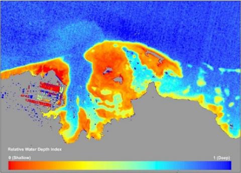
The topographic conditions of the shallow waters of Gili Sumber Kima are divided into four morphological forms of coral reef, namely reef flat, reef crest, fore reef, and patch reef. Reef flats are dominated by substrate, seagrass, and macroalgae, while reef crests, fore reefs, and patch reefs are dominated by coral reefs. These forms can be identified by calculating and characterizing the depth of the coastal waters. The spatial data on water depth, or commonly called bathymetry, can be extracted from remote sensing imagery using various modeling methods. These methods rely on primary data (measurement in the field) and/or qualitative estimates, which are based on the characteristics of the depth range identifiable from remote sensing images. Bathymetry modeling can be performed using many techniques, including band ratio, single band, and Relative Water Depth Index (RWDI) [51]. Because the bathymetry information is not available in the study area, single band and band ratio are therefore inapplicable. To produce the spatial data of relative bathymetry, the research employed RWDI. The principle of RWDI is the spectral response of objects at the bottom of the water to visible and near-infrared channels. RWDI produces bathymetry with relative depth information, as indicated by the ratio of 0 (shallow waters) and 1 (deep waters) [52]. The bathymetry model showed that shallow waters dominated the coastal waters of Gili Sumber Kima. The shallow waters are shown in red to yellow, while deep waters are depicted in cyan to bluish color (Figure 10).

10.jpg

Figure 10. Relative water depth index (RWDI) map

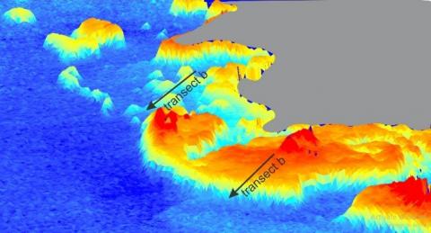
The 3-dimensional visualization proved that the bathymetry model corresponded to the actual depth in the field. There were slightly different morphological appearances in the 3-dimensional view of the eastern waters. Patch reefs, where coral reefs grew, were dominant in these waters. Topographically, their form resembled small hills that were separated from each other (Figure 11). There was a slight error in the modeling results, especially on a small island in the middle of the shallow water. The waters around the small island had a very clean sand substrate, and the field survey showed that they were 0.3 to 1 m in depth. However, because the pixel values were severely bright, the RWDI model read these features as very shallow waters. Another error was found in waters with depths of >10 m because the RWDI model read these features as the saturation of the pixel values. If viewed from satellite images, deep waters produce a similar spectral response. In this case, the RWDI model reads the response as saturation and perceives the pixel values as having a relatively similar depth (1).

11.jpg

Figure 11. 3D Visualization of RWDI Bathymetry

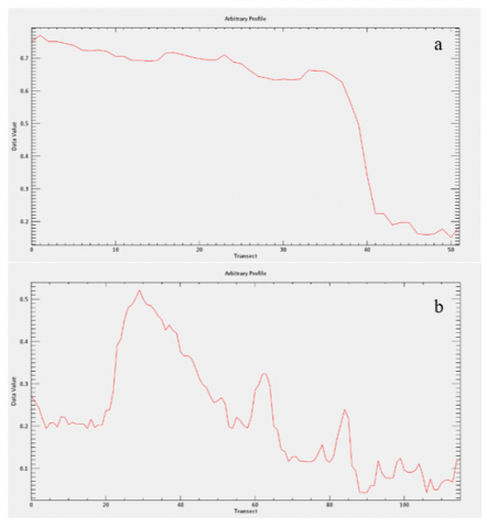
The cross-sectional profile of the modeled bathymetry (Figure 12) was formed with a transect from shallow to deep waters. It depicted the topographical conditions of this segment. In this study, the transect was an imaginary line cutting through the northern part of the shallow waters in Gili Sumber Kima, as shown in Figure 11. This part of the waters was selected because the field survey was carried out intensively in this location. In other words, verifying the results of the modeling with the actual conditions would be straightforward. The cross-sectional profile of the bathymetry of shallow waters in Gili Sumber Kima is presented in Figure 12.

12.png

Figure 12. Bathymetry cross-profile: a) transect a and b) transect b

According to the cross-sectional profile, the morphological zonation of the coral reefs is in line with the discussion at the beginning of Point 3.4. The morphology is divided into four forms, namely reef flat, reef crest, fore reef, and patch reef. Reef flats have a relatively flat topography, while reef crests are the transition zone between reef flats and deep waters (cliff). Fore reefs are indicated by steep topography overlooking open sea waters. Patch reefs have similar topography to a small hill with a hilltop that is not too high (Figure 11). So far, bathymetry mapping using remote sensing imagery has been able to produce accurate data, with the standard errors ranging between 0.79 and 1.05 m [53-55]. The spatial information of bathymetry is essential in coastal area management and planning. Bathymetry shows which waters have the potential for fisheries using the habitat approach. Also, it functions as supporting data in navigation and port development plans and identifies safe locations for the ship’s mooring. Therefore, rapid acquisition of bathymetric data from remote sensing imagery is one of the breakthroughs in coastal area management and development.