Lingyan Ou![]() | Yu Li
| Yu Li![]() | Wanyong Jiang*
| Wanyong Jiang*![]()
© 2025 The authors. This article is published by IIETA and is licensed under the CC BY 4.0 license (http://creativecommons.org/licenses/by/4.0/).
OPEN ACCESS
The ongoing transition toward low-carbon energy and the rapid development of carbon trading markets are reshaping multi-regional energy systems. These systems are increasingly characterized by cross-regional interconnection and multi-energy collaboration. However, existing optimization models often oversimplify thermal networks and treat carbon pricing as an exogenous constraint, limiting their ability to reveal how carbon policies influence energy flows through physical infrastructures. This study proposes a two-stage thermodynamics-economics coupled optimization framework. The first stage focuses on minimizing total heat supply and distribution losses by optimizing supply temperatures under fixed flow conditions, based on a detailed thermal power flow model. The second stage integrates electricity, heat, and gas systems into a unified dispatch model that minimizes total operational and carbon trading costs. Carbon price signals are embedded into decision-making, enabling quantitative analysis of their impact on generation scheduling and interregional energy exchange. The proposed model establishes a clear path from physical efficiency to economic coordination, offering a systematic and scalable approach for evaluating carbon trading policies in complex energy networks.
multi-regional energy systems, carbon trading policy, thermodynamic analysis, collaborative optimization, thermal power flow
The global energy transition is currently at a critical juncture [1-3]. Building a clean, low-carbon, secure, and efficient energy system has become an inevitable choice to address climate change and ensure energy security [4-6]. Against this backdrop, multi-regional energy systems have attracted growing attention as a technological paradigm capable of achieving multi-energy complementarity and synergistic efficiency improvements [7, 8]. In particular, interconnected regional energy systems enable the spatial and temporal redistribution of energy, which helps smooth out the variability of renewable energy sources and enhances the overall efficiency of energy utilization.
At the same time, the carbon trading market has emerged as a key market-oriented emission reduction mechanism [9, 10], fundamentally reshaping the operational logic and planning decisions of energy systems by assigning a price to carbon emissions. This mechanism internalizes the environmental externalities of carbon emissions into economic costs, compelling energy systems to pursue decarbonization while satisfying energy demand. However, the physical operation of energy systems is inherently governed by the laws of thermodynamics [11], while their economic decisions are subject to market mechanisms and policy constraints [12]. Therefore, the development of a collaborative optimization model that can accurately represent both the thermodynamic characteristics of multi-regional energy transfer and the economic incentives of carbon trading is of critical significance for understanding and guiding the low-carbon transformation of energy systems.
This study proposes a thermodynamics- and economics-based collaborative optimization model for multi-regional energy systems, with a focus on the systematic evaluation of carbon trading policies. The significance of this work lies in two main aspects. Theoretically, it advances energy system modeling by deeply integrating physical constraints such as thermal power flow and multi-regional coupling with economic objectives such as carbon trading costs. This provides a new analytical framework for understanding the complex interactions between physical and economic layers in energy systems. Practically, the proposed model serves as a scientific decision-making tool for system operators, planners, and policymakers. By simulating system operations under various carbon pricing scenarios, the model enables a quantitative evaluation of the emission reduction effectiveness and economic impacts of carbon trading policies, identifies key technical bottlenecks and potentials for cross-regional coordination, and offers robust analytical support for optimizing carbon market design, developing efficient emission reduction strategies, and enhancing interregional energy infrastructure connectivity.
Although considerable progress has been made in optimizing multi-regional energy systems, several notable limitations persist in existing methodologies. First, many studies [13-15] oversimplify thermal network modeling by neglecting the dynamic hydraulic-thermal coupling and transmission delays, or by adopting overly idealized assumptions such as constant heat loss coefficients, which significantly compromise the physical accuracy of optimization results, as pointed out in reference [16]. Second, when addressing carbon trading policies, a large number of studies [17-19] treat them as exogenous constraints or linear cost functions, failing to reveal the intrinsic mechanisms by which carbon price signals interact with equipment operation constraints and network transmission limits to influence energy flows and carbon footprints across regions, a limitation also noted in reference [20]. Lastly, most models [21, 22] lack a closed-loop framework that bridges the physical and economic layers. Specifically, they fail to first establish a thermodynamically optimal baseline for energy supply, upon which the economic effects of carbon pricing can be evaluated. As a result, these models are unable to accurately distinguish between policy impacts and the inherent physical potential of the system.
To address the above limitations, this study conducts research in two core areas. The first focuses on optimizing the heat supply from multi-regional heat sources. This part centers on the thermodynamic foundation of the system and sequentially performs multi-regional thermal power flow analysis and determination of initial flow rates. The objective is to minimize the total system heat supply, thereby establishing a physically compliant, low-loss baseline plan for thermal energy distribution. The second part addresses the collaborative optimization of multi-regional energy systems. Using the optimal heat supply obtained from the first stage as a key input, a coupled electricity-heat-gas optimization model is developed to minimize the sum of operational and carbon trading costs. This allows for a comprehensive analysis of the effects of carbon trading policies on unit dispatch, interregional energy flows, and total emissions.
The central value of this research lies in the proposed two-stage "physics-first, economics-driven" collaborative optimization framework. By strictly adhering to thermodynamic laws, the model ensures the physical feasibility of the optimized solutions, while also systematically embedding carbon trading policies into economic decision-making. As such, the proposed framework offers a complete and reliable theoretical and methodological foundation for the refined design and implementation of carbon trading policies in complex multi-regional energy systems.
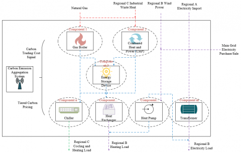
The collaborative optimization framework proposed in this study aims to overcome the limitations of traditional single-region energy systems by integrating thermodynamic principles with economic theory to systematically assess the deeper impacts of carbon trading policies on multi-regional energy allocation. The structure of the framework is illustrated in Figure 1. This framework tightly integrates physical constraints and market mechanisms. On the physical side, it relies on the laws of thermodynamics to accurately quantify energy quality loss and temperature dynamics during interregional energy transmission and conversion processes. Special attention is given to thermal transfer efficiency and temperature decay across regional heating networks. On the economic side, the framework introduces carbon trading costs as a critical variable, converting emission allowances into explicit economic costs. This enables the optimization process to consider not only traditional economic factors such as energy procurement and equipment operation and maintenance (O&M), but also to internalize environmental externalities into system-level decision-making.
Figure 1. Collaborative optimization framework for multi-regional integrated energy systems under carbon trading policies
By constructing a dual-constraint model that incorporates both physical and economic factors, the framework achieves collaborative optimization across energy production, transmission, and consumption at a multi-regional scale. It ensures that regional energy demand is met while enabling carbon flow tracking and delivering precise evaluations of the economic and environmental benefits of carbon policies.
This optimization framework adopts a multi-stage structure. The first stage focuses on thermodynamics-based optimization of regional energy flows. It centers on a multi-regional hydraulic-thermal coupling model of district heating networks. By fixing flow rates and optimizing temperature strategies, the model enables a linearized treatment of thermal power flows. This ensures the diversified heat load demands across regions are satisfied while minimizing total heat supply and network losses. This stage primarily addresses the modeling complexities arising from thermal inertia and transmission delays in multi-regional networks.
The second stage performs economic and environmental co-optimization driven by carbon trading policies. The total regional heat supply and electric load obtained from the first stage are used as boundary conditions. A multi-objective optimization model is constructed to minimize both total operating cost and carbon emissions. A tiered carbon pricing mechanism and interregional emission allowance trading rules are incorporated to dynamically balance the operational strategies of gas turbines, heat pumps, and other electricity-heat coupled devices during dispatch. The result is an energy scheduling plan that achieves both thermodynamic efficiency and carbon economic feasibility across regions.
Through this two-stage iterative optimization, the proposed framework establishes a closed-loop feedback mechanism from the physical layer to the decision-making layer. It provides a comprehensive modeling paradigm for the systematic analysis of carbon trading policy impacts in the context of coordinated regional emission reductions.
2.1 Optimization of multi-regional heat supply dispatch
The core distinction between a multi-regional and a single-region energy system lies in the significant energy losses and dynamic delays during spatial energy transmission. Ignoring these physical realities renders any economic optimization fundamentally unsound. From the perspective of economics and carbon trading systems, minimizing total heat supply directly corresponds to reducing the consumption of primary energy—especially in systems where gas boilers or combined heat and power (CHP) units serve as primary heat sources. This reduction translates into decreased fossil fuel usage, such as natural gas, thereby lowering the “physical baseline” of carbon emissions at the source. The minimized heat supply becomes the reference for calculating carbon emissions and trading costs in subsequent environmental-economic optimization. Without this thermodynamically grounded baseline, carbon cost accounting may rely on energy supply schemes already plagued by inefficiencies, leading to serious distortions in policy signaling.
To establish a physically consistent, efficient, and accurate energy supply baseline for subsequent carbon-trading-integrated economic optimization, this study first performs optimization of heat supply dispatch across multiple regions. This preliminary step, rooted in thermodynamic first principles, addresses the foundational issue of interregional energy coordination.
The first step—multi-regional thermal power flow analysis—aims to accurately capture temperature degradation and pressure drops resulting from pipe heat loss and hydraulic conditions during the transmission of heat from sources to loads. Essentially, this step applies the second law of thermodynamics to pipeline systems, quantifying both the "quality" and "quantity" loss of energy.
The second step—determination of regional initial flow rates—uses hydraulic calculations to establish a stable and efficient transport medium based on the power flow analysis. By fixing mass flow rates, the complex nonlinear optimization problem is converted into a linear form, focusing dynamic system variables on supply and return temperatures. This greatly simplifies the model while preserving its physical fidelity.
The third and final step—minimization of multi-regional heat supply—naturally follows: based on accurate knowledge of network losses and a stable flow structure, the model optimizes the dispatch timing and supply temperatures of all heat sources such that the total thermal energy injected to meet end-use demand is minimized. The following provides a detailed analysis of these three steps.
From a systematic perspective grounded in economics and carbon trading policies, heat supplied in one region may originate from local gas boilers, remote CHP plants, or industrial waste heat. Thermal power flow analysis enables tracing the source, path, and associated transmission losses of every gigajoule of heat. This ensures that the carbon responsibility of consumed heat can be fairly and accurately allocated to its producer—a prerequisite for any emissions trading mechanism. The thermal power flow analysis in this study is grounded in thermodynamic laws and aims to construct a physically realistic model for subsequent economic and carbon optimization. It rigorously follows the principles of energy conservation and entropy degradation, employing a coupled hydraulic-thermal modeling framework to simulate the spatiotemporal distribution and degradation of heat within large-scale networks.
Hydraulic analysis ensures the feasibility of heat delivery, analogous to Kirchhoff’s current law in electrical circuits, mandating mass flow balance at each node. This determines flow paths and physical constraints for the thermal medium. Thermal analysis quantifies energy loss in terms of both quality and quantity:
·Node thermal power balance links supply and demand;
·Pipe temperature drop models, based on heat transfer theory, quantify temperature degradation caused by heat loss—directly reflecting the second law of thermodynamics and revealing the physical path and extent of energy loss;
·Hydraulic mixing temperature models compute node temperatures when branches of different flow rates and temperatures converge, ensuring accurate tracking of energy quality (exergy) across interconnected regions.
Specifically, let the network incidence matrix be denoted by Xg, mass flow rate in each pipe by l, and node-level mass flow rates by lw. The node-level hydraulic balance is given by:
${{X}_{g}}l={{l}_{w}}$ (1)
Let the thermal power consumption at each node be ψ, specific heat of water be zo, supply temperature be St, and return temperature be Sp. The thermal power at each node is calculated as:
$\psi ={{z}_{o}}{{\dot{l}}_{q}}\left( {{S}_{t}}-{{S}_{p}} \right)$ (2)
Let the inlet and outlet temperatures of a pipe segment be SQS and SEND, ambient temperature be Sx, heat transfer coefficient be η, and pipe length be M. The pipe temperature drop is given by:
${{S}_{END}}=\left( {{S}_{QS}}-{{S}_{x}} \right){{r}^{\frac{-\eta M}{{{z}_{o}}\dot{l}}}}+{{S}_{x}}$ (3)
Let the mass flow rate of the inflow and outflow pipe segments be lIN and lOUT, the node outlet temperature be SOUT, and the inflow segment end temperature be SIN. The hydraulic mixing temperature is computed as:
$\left( \sum{{{l}_{OUT}}} \right){{S}_{OUT}}=\sum{\left( {{l}_{IN}}{{S}_{IN}} \right)}$ (4)
From a systems economics and carbon trading policy standpoint, the determination of initial flow rates forms a crucial bridge between physical baselines and economic policy modeling. It directly affects the operational energy efficiency and the baseline carbon footprint of the entire network. Pipe flow rates critically influence temperature losses, and any heat lost in transit must be compensated by additional fuel combustion at the source. By scientifically determining and constraining these initial flow rates, the system minimizes avoidable transmission losses and reduces the basic dependence on fossil fuels—effectively lowering the physical baseline of emissions.
The core logic of determining regional initial flow rates is as follows: under an ideal lossless assumption, the minimum theoretical flow rate l0u needed to satisfy the thermal demand of each regional node—given the designed temperature differential—can be computed. This set of initial flow rates forms the "demand-side baseline" for hydraulic distribution, ensuring that optimization begins from a feasible point that satisfies basic user energy needs. Let Mu denote the length of pipe u, and γu its heat loss coefficient. The heat loss objective function for the network is:
$MIN{{D}_{1}}=MIN\left( \sum\limits_{u=1}^{v}{{{M}_{u}}{{\gamma }_{u}}} \right)$ (5)
However, real-world pipeline systems inevitably suffer from heat loss due to the second law of thermodynamics. Therefore, initial flow determination does not stop at idealized calculations but incorporates these as hard constraints into the actual network model. By enforcing "pipe flow rate not less than l0u" as a constraint, and combining it with node-level mass balance, a hydraulically feasible flow allocation scheme is constructed. Let the upper and lower bounds of pipe u's flow rate be lu,MAX and lu,MIN, the flow balance and pipe flow constraints are:
${{l}_{u,MIN}}\le {{l}_{u}}\le {{l}_{u,MAX}}$ (6)
The heat loss coefficient γᵤ for each pipe segment is calculated by:
${{\gamma }_{u}}=1-{{r}^{-\eta {{M}_{u}}/\left( {{z}_{o}}{{{\dot{l}}}_{u}} \right)}}$ (7)
This formulation ensures that, even under real-world heat loss, sufficient thermal medium is delivered to the load points to compensate for transmission losses and satisfy user demand. This physically grounded setup stabilizes the hydraulic layer of the thermal-hydraulic coupling, laying a solid foundation for the subsequent accurate computation of thermal losses and heat supply optimization.
The final stage—minimization of total heat supply—seeks the thermodynamic efficiency limit of the system under the previously established hydraulic distribution and thermal flow analysis. From a carbon trading policy perspective, identifying this minimum total supply is fundamental, as it defines the lower bound of carbon emissions at the physical level. Since total heat supply directly correlates with the fuel consumption of gas boilers and CHP units, minimizing it reduces fossil fuel consumption and direct emissions at the source. Under constraints such as pipe flow rates, return temperature, and supply temperature bounds, the optimization adjusts the supply temperatures of each heat source to deliver the exact amount of high-grade thermal energy required to offset both transmission losses and end-user demands. This approach reflects the essence of the second law of thermodynamics—by minimizing unnecessary transmission of high-exergy energy and large temperature drops, it reduces exergy destruction due to irreversible heat transfer. Let St,MAX and St,MIN denote the upper and lower limits of supply temperature, and lt, l1the flow rates in source-load connecting pipelines. The optimization objective is formulated as:
$\begin{aligned} & M I N D_2=z_o l_t\left(S_t-S_p\right) \\ & \text { s.t. }\left\{\begin{array}{l}S_{t, M N D} \leq S_t \leq S_{t, M A X} \\ S_{E N D}=\left(S_{Q S}-T_x\right) r^{\frac{-\eta M}{z o i}+S_x} \\ \psi_1=z_o l_1\left(S_t-S_p\right)\end{array}\right.\end{aligned}$ (8)
2.2 Multi-regional energy co-optimization
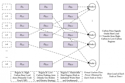
Figure 2 depicts the mechanistic model by which a carbon trading policy systematically influences multi-regional energy dispatch decisions. The concepts of carbon trading policy and carbon-flow tracing are introduced, and regions are classified by energy mix and carbon intensity so that the heterogeneity across “multi-regions” becomes visible in the co-optimization process. Unlike conventional coordinated scheduling that focuses solely on thermal flows, the proposed model presents physical thermal flows alongside virtual carbon/cost flows, linking physical heat-flow information to the economic signal of carbon trading costs. As shown schematically, carbon pricing creates cost differentials among heat sources with different carbon intensities, thereby reshaping optimal decisions: load centers are steered to prioritize low‑carbon regional heat, ultimately minimizing the sum of economic and environmental costs.
To capture the dual constraints and incentives faced by modern energy systems, the co-optimization model jointly considers operating cost and carbon trading cost, enabling a systematic evaluation of carbon trading policies. Operating cost reflects the traditional economic dimension required for financial viability. However, minimizing operating cost alone tends to lock in high‑carbon pathways, as systems may favor inexpensive fossil fuels while overlooking environmental externalities. Introducing carbon trading costs is therefore essential: by internalizing emissions as explicit, quantifiable financial obligations, the model alters the relative cost competitiveness of technologies within the objective function. The optimizer must weigh “low operating cost but high carbon cost” for fossil options against “higher operating cost but lower carbon cost” for cleaner options, thereby inducing a spontaneous shift toward low‑carbon dispatch—faithfully representing carbon trading as an economic lever.
Figure 2. Schematic of coordinated thermal dispatch and carbon-flow tracing under a carbon trading regime
The operating cost objective aggregates six components: coal‑fired generation cost, natural gas cost, equipment O&M cost, (duplicate line intentionally preserved as in the source) equipment O&M cost, carbon sequestration cost, and cost of purchasing CO₂ allowances from the market. The objective is:
${{D}_{1}}=\sum\limits_{s=1}^{24}{\left[ \begin{align} & {{D}_{CAP}}\left( s \right)+{{D}_{GAS}}\left( t \right)+{{D}_{GR}}\left( s \right)+{{D}_{pl}}\left( s \right) \\ & +{{D}_{z,SEQ}}\left( s \right)+{{D}_{z,BUY}}\left( s \right) \\ \end{align} \right]}$ (9)
Here, the coal‑fired generation cost DCAP reflects the true economic burden of high‑carbon generation in a market environment. Thermodynamically, coal units convert the fuel’s chemical energy into electricity and heat; conversion efficiency determines fuel consumption and thus baseline fuel expenditure. Without environmental costs, low fuel prices could make coal appear cost‑competitive. Under carbon trading, however, DCAP becomes the “baseline load” for subsequent carbon cost accounting: given its high carbon intensity, coal consumes a substantial share of allowances or bears significant carbon cost. Let x, y, and z denote fuel cost coefficients; DCAP is computed as:
${{D}_{CAP}}\left( s \right)=x\times {{O}_{CAP}}{{\left( s \right)}^{2}}+y\times {{O}_{CAP}}\left( s \right)+z$ (10)
Introducing natural gas cost captures the transitional role of a relatively lower‑carbon fossil fuel. Thermodynamically, gas‑fired CHP or boilers typically achieve higher conversion efficiencies than coal, implying lower exergy destruction and fuel use per unit of useful energy. Economically, gas cost represents the direct outlay for an alternative fossil pathway. Including this term allows explicit comparison of “coal versus gas” within the multi‑regional model. Under carbon trading, gas still emits CO₂ but at a lower intensity than coal, so optimizing coal and gas jointly reveals how carbon price shifts their relative competitiveness—e.g., higher carbon prices push the system toward gas due to its lower per‑unit carbon cost. Let the gas purchase price be OGA; the gas cost DGAS is:
${{D}_{GAS}}\left( s \right)=\left[ {{N}_{HS}}\left( s \right)+{{N}_{HY}}\left( s \right)-{{N}_{P2G}}\left( s \right) \right]{{O}_{GA}}$ (11)
The power purchase cost quantifies the direct expenditure of exchanging energy with the upstream grid and forms a key market boundary for system economics. It is essentially the time‑sum of purchased energy multiplied by nodal time‑of‑use prices. This enables economic trade‑offs between self‑supply and external purchases. From a carbon trading perspective, the implicit carbon flow of purchased electricity must also be accounted for: when the marginal cost of self‑generation exceeds the all‑in cost of imports, the model may increase purchases, lowering operating outlays but altering the system’s total carbon footprint via the grid’s emission factor—thereby affecting allowance balances and carbon cost. Let OGB(s) be purchased energy and OGR(s) the time‑of‑use price at time s; the cost DGD is:
${{D}_{GR}}\left( s \right)={{O}_{GB}}\left( s \right){{O}_{GR}}\left( s \right)$ (12)
Accounting for equipment O&M cost follows a life‑cycle economic rationale, ensuring engineering practicality and long‑term sustainability. Coal units, gas turbines, heat pumps, and network assets incur wear, aging, and maintenance expenses. Operating conditions—shaped by system‑level dispatch—directly influence O&M cost. Ignoring O&M may bias the model toward frequent cycling or inefficient operating zones, superficially reducing fuel cost while increasing total cost and harming asset life. Incorporating O&M extends beyond variable costs to include strategy‑dependent capital wear, providing a realistic baseline to assess the full economic impact of carbon policies. Let device output be Ou and the O&M cost coefficient be Jpl; the O&M cost Dpl is:
${{D}_{pl}}\left( s \right)={{O}_{u}}{{J}_{pl}}$ (13)
Introducing carbon sequestration cost provides an active end‑of‑pipe abatement option that broadens the policy response toolkit by extending system boundaries from “energy conversion—emissions—capture and storage.” CCS consumes additional energy for separation, compression, and transport, reducing net output and increasing equivalent fuel cost. In economic terms, sequestration cost quantifies this abatement expense. When the market carbon price exceeds the marginal cost of sequestration, the optimizer favors CCS; otherwise, it purchases allowances. Let ηz.SEQ be the CO₂ transport and storage cost coefficient; the sequestration cost Dz.SEQ is:
${{D}_{z,SEQ}}\left( s \right)={{\eta }_{z,SEQ}}\sum\limits_{s=1}^{24}{{{W}_{SEQ,Z{{P}_{2}}}}\left( s \right)}$ (14)
Including the cost of purchasing CO₂ allowances reflects the core market mechanism—compliance via trading. This term represents the option to buy allowances rather than abate when internal marginal abatement cost is higher than the allowance price. Within a multi‑regional framework, this enables coordinated optimization of carbon costs across regions: one region may sell surplus allowances, while another purchases to sustain necessary high‑emission production. Thus, the model captures how the market allocates scarce emission rights efficiently across regions. Let ηz.BUY be the CO₂ purchase price and WBUY,ZP2,(s) the purchased quantity; the cost is:
${{D}_{z,BUY}}\left( s \right)={{\eta }_{z,BUY}}\sum\limits_{s=1}^{24}{{{W}_{BUY,Z{{P}_{2}}}}\left( s \right)}$ (15)
Combining the six components into a unified operating‑cost objective yields a decision environment that fully responds to carbon price signals. The composite objective no longer targets only traditional procurement and maintenance minimization; it internalizes carbon trading as a core decision variable, forcing simultaneous consideration of direct expenditures and compliance costs at every dispatch step. This structure reveals the interaction among carbon price, fuel prices, and technology costs, including the thresholds at which strategies shift from “buy allowances,” to “invest in CCS,” and eventually to “fully transition to renewables.”
For the carbon trading cost objective, the model first assigns free allowances to the system, emulating common real‑world practices (e.g., grandfathering or benchmark allocation) to set a fair and operational starting point. Economically, free allocation tempers initial compliance shocks, improving policy feasibility. In the multi‑regional model, free allocation to each region or major emitter establishes a “carbon budget.” Let σCAP, σHS and σHYdenote allowance coefficients for coal units, gas turbines, and gas boilers, respectively, and OHS(s), OHY(s) their time‑indexed outputs; then
$\left\{ \begin{align} & {{R}_{CAP,x}}\left( s \right)={{\sigma }_{CAP}}{{O}_{CAP}}\left( s \right) \\ & {{R}_{HS,x}}\left( s \right)={{\sigma }_{HS}}{{O}_{HS}}\left( s \right) \\ & {{R}_{HY,x}}\left( s \right)={{\sigma }_{HY}}{{O}_{HY}}\left( s \right) \\ \end{align} \right.$ (16)
Summing individual allocations yields the system‑wide cap, i.e., a policy‑driven upper bound on emissions. This cap is the key lever in cap‑and‑trade, creating scarcity in emission rights. Varying the cap level enables analysis of how policy stringency affects operating strategies, total cost, and interregional energy flows. The system cap is:
${{R}_{TO}}\left( s \right)={{R}_{CAP,x}}\left( s \right)+{{R}_{HS,x}}\left( s \right)+{{R}_{HY,x}}\left( s \right)+{{R}_{GR,x}}\left( s \right)$ (17)
By mass conservation and stoichiometry, decision variables map to emissions via fuel‑specific emission factors, computed by device and by region. Let εHS and εHY be emission factors for gas turbines and gas boilers, and εGR the emission factor for purchased electricity; then
$\left\{ \begin{align} & {{Z}_{HS,x}}\left( s \right)={{\varepsilon }_{HS}}{{O}_{HS}}\left( s \right) \\ & {{Z}_{HY,x}}\left( s \right)={{\varepsilon }_{HY}}{{O}_{HY}}\left( s \right) \\ & {{Z}_{GD,x}}\left( s \right)={{\varepsilon }_{GD}}{{O}_{GR}}\left( s \right) \\ \end{align} \right.$ (18)
Aggregating emissions across devices and regions gives total system emissions, a quantity directly comparable to the cap. This comparison triggers trading behavior: if total emissions are below the cap, the system is a net seller of allowances and earns revenue; otherwise, it is a buyer and incurs cost. This accounting links physical emissions to market outcomes:
${{Z}_{TO}}\left( s \right)=W_{CAP,Z{{P}_{2}}}^{F}\left( s \right)+{{Z}_{HS,x}}\left( s \right)+{{Z}_{HY,x}}\left( s \right)+{{Z}_{GR,x}}\left( s \right)$ (19)
Eq. (20) defines the net trading volume of emission rights as the difference between total emissions and the system cap, with sign indicating net purchase (positive) or net sale (negative). While (20) represents the system’s net position with the external market, the model can also emulate interregional trades internally; the net value summarizes all internal and external transactions and reflects compliance status under carbon constraints:
${{S}_{TO}}\left( s \right)={{Z}_{TO}}\left( s \right)-{{R}_{TO}}\left( s \right)$ (20)
Let η denote the baseline carbon price, m the price‑tier interval, β the increment per tier, and σ the abatement compensation coefficient. The carbon trading cost—which completes the internalization of environmental externalities into explicit, quantifiable cost—is:
${{D}_{2}}=\left\{ \begin{align} & \eta \left( 1+4\sigma \right){{S}_{TO}},{{S}_{TO}}<-3m \\ & \eta \left( 1+3\sigma \right){{S}_{TO}},-3m\le {{S}_{TO}}<-2m \\ & \eta \left( 1+2\sigma \right){{S}_{TO}},-2m\le {{S}_{TO}}<-m \\ & \eta \left( 1+\sigma \right){{S}_{TO}},-m\le {{S}_{TO}}<0 \\ & \eta {{S}_{TO}},0\le {{S}_{TO}}<m \\ & \eta \left( 1+\beta \right)\left( {{S}_{TO}}-m \right)+\eta \left( 1+\beta \right)m,m\le {{S}_{TO}}<2m \\ & \eta \left( 1+2\beta \right)\left( {{S}_{TO}}-2m \right)+\eta \left( 2+2\beta \right)m,2m\le {{S}_{TO}}<3m \\ & \eta \left( 1+3\beta \right)\left( {{S}_{TO}}-3m \right)+\mu \left( 3+3\beta \right)m,3m\le {{S}_{TO}} \\ \end{align} \right.$ (21)
Here, the carbon price is a core policy variable determining the economic penalty of emissions. With this cost term, carbon trading ceases to be an exogenous, vague constraint and becomes a concrete component of the objective, co‑optimized alongside fuel and O&M costs.
Finally, the total optimization objective includes both carbon trading and operating costs to realize genuine economic-environmental co‑optimization. Each dispatch decision simultaneously weighs direct economic outlays and compliance costs:
$D=MIN\left( {{D}_{1}}+{{D}_{2}} \right)$ (22)
The model constraints fall into the following categories:
1) Load balance constraints.
At every time and in every region, the sum of electric and thermal outputs must meet the corresponding loads. This guarantees physical feasibility and fixes demand so that differences across carbon pricing scenarios arise purely from supply‑side shifts, clarifying how carbon trading drives low‑carbon transitions. Let MLO(s) and OLO(s) denote thermal and electric loads; OHS,g(s) and OHY(s) denote thermal outputs of gas turbines and gas boilers; OHS,r(s) and OQS(t) denote electric outputs of gas turbines and wind units. Then
$\begin{align} & {{M}_{LO}}\left( s \right)={{O}_{HS,g}}\left( s \right)+{{O}_{HY}}\left( s \right) \\ & {{O}_{LO}}\left( s \right)={{O}_{CAP,r,TO}}\left( s \right)+{{O}_{HS,r}}\left( s \right)+{{O}_{QS}}\left( s \right)+{{O}_{GR}}\left( s \right) \\ \end{align}$ (23)
2) Device operating constraints.
These capture thermodynamic characteristics and operational flexibility (e.g., the energy‑consumption-capture‑rate curve of CCS plants, the conversion efficiency and cycling limits of P2G). They translate physical limits and dynamics into mathematical bounds so that dispatch instructions are technically implementable. Carbon prices influence these operating states—higher prices incentivize CCS loading and P2G absorption of renewables. Let O(s) and O(s-1) denote device outputs at time s and s−1, and EUP and EDO the ramp‑up and ramp‑down limits; then
$-{{E}_{DO}}<O\left( s \right)-O\left( s-1 \right)<{{E}_{UP}}$ (24)
3) Unit output constraints.
Lower bounds reflect minimum stable generation; upper bounds are rated capacities. These limits shape system flexibility and marginal abatement cost, especially under load fluctuations. The constraints are:
$\left\{ \begin{align} & 0<{{O}_{QS}}<{{O}_{QS,MAX}} \\ & {{O}_{HS,MIN}}<{{O}_{HS}}<{{O}_{HS,MAX}} \\ & {{O}_{CAP,MIN}}<{{O}_{CAP}}<{{O}_{CAP,MAX}} \\ & {{O}_{HY,MIN}}<{{O}_{HY}}<{{O}_{HY,MAX}} \\ & 0<{{O}_{O2H}}<{{O}_{O2H,MAX}} \\ \end{align} \right.$ (25)
4) Interconnector constraints.
These define the spatial dimension of the model by limiting interregional power transfer capacities. They determine the physical feasibility of shifting carbon responsibility across space. Under carbon trading, heterogeneous marginal abatement costs across regions interact with transfer limits to shape optimal cross‑regional coordination. The constraints are:
${{d}_{u,k,MIN}}\le {{d}_{u,k}}\le {{d}_{u,k,MAX}}$ (26)
5) Natural gas system constraints.
A physically consistent gas network—parallel to the power and heat networks—is modeled per fluid mechanics to ensure hydraulic feasibility and safety. As the hub of power-gas-heat coupling, gas network capability and dynamics affect dispatchability of gas‑linked devices and the integration of P2G production and storage. Let Xh be the gas‑network incidence matrix, d the segment mass flow, and dw the nodal mass flow; nodal flow balance is:
${{X}_{h}}d={{d}_{w}}$ (27)
Let de be steady‑state segment flow, Je the pipeline constant, and tuk the flow direction; the pressure-flow relation is:
${{d}_{e}}={{J}_{e}}{{t}_{uk}}\sqrt{{{t}_{uk}}\left( o_{u}^{2}-o_{k}^{2} \right)}$ (28)
Let nodal pressure bounds be ou,MAX and ou,MIN; the nodal pressure constraint is:
${{o}_{u,MIN}}\le {{o}_{u}}\le {{o}_{u,MAX}}$ (29)
Let gas‑well output bounds be dt,MAX and dt,MIN; the gas‑supply constraint is:
${{d}_{t,MIN}}\le {{d}_{t}}\le {{d}_{t,MAX}}$ (30)
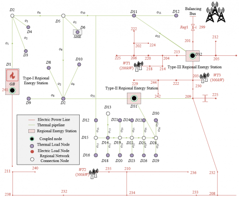
A test system comprising three representative energy regions is constructed, interconnected via power and district heating networks. Region A is equipped with coal-fired CHP units characterized by high carbon emissions and serves as the base-load energy provider. Region B primarily relies on gas boilers and wind power for flexible, low-carbon supply. Region C is rich in zero-carbon industrial waste heat. Interregional energy exchange is enabled through power interconnectors and cross-regional heating pipelines. Coupling technologies, such as power-to-gas (P2G) and carbon capture systems, are deployed at key nodes. The schematic layout of the test system is shown in Figure 3.
Figure 3. Topological structure of the test case for the multi-regional energy system
To systematically assess the operational impact of different carbon trading policy types, relevant experiments were conducted. Table 1 presents the results. Comparing the base case with fixed carbon price and tiered carbon price scenarios reveals that introducing carbon trading significantly alters the system’s economic operation. Under the fixed carbon price scenario, total system operating cost decreased by 16.7% and carbon emissions by 9.7%, indicating that internalizing carbon costs compels the system to adjust unit commitment and increase low-carbon output. In the tiered carbon price scenario, the system achieved ¥128,745 in carbon revenue and further reduced total cost to ¥1,378,852, with a 21.4% reduction in carbon emissions. This tiered incentive mechanism activates deeper emission reduction potential, prompting the system to seek cost-optimal low-carbon strategies while satisfying energy demand. The results suggest that carbon trading policies—especially tiered pricing mechanisms—effectively guide shifts in system dispatch strategies, enhancing both economic performance and environmental sustainability, with tiered pricing outperforming flat pricing in incentive effectiveness.
Table 1. Comparison of optimization results under different types of carbon trading policies
|
Indicator |
Scenario 1: Baseline |
Scenario 2: Fixed Carbon Price |
Scenario 3: Tiered Carbon Price |
|
Economic Indicators (CNY) |
|||
|
Electricity Purchase Cost |
353,725 |
315,871 |
285,634 |
|
Natural Gas Purchase Cost |
933,034 |
967,346 |
1,025,683 |
|
Coal-Fired Unit Cost |
208,527 |
205,971 |
185,324 |
|
Wind and Solar Curtailment Penalty |
12,216 |
11,488 |
8,956 |
|
Carbon Trading Cost |
0 |
52,880 |
-128,745* |
|
Total System Operating Cost |
1,815,032 |
1,512,367 |
1,378,852 |
|
Environmental Indicators |
|||
|
Total System Carbon Emissions (t) |
2,704 |
2,442 |
2,125 |
|
Carbon Intensity (kgCO₂/CNY) |
1.49 |
1.61 |
1.54 |
Table 2. Comparison of optimization results between coordinated and independent multi-regional operation
|
Indicator |
Scenario 4: Independent Operation + Tiered Carbon Price |
Scenario 5: Regional Coordination + Tiered Carbon Price |
|
Economic Indicators (CNY) |
||
|
Electricity Purchase Cost |
285,634 |
242,107 |
|
Natural Gas Purchase Cost |
1,025,683 |
892,451 |
|
Coal-Fired Unit Cost |
185,324 |
165,892 |
|
Wind and Solar Curtailment Penalty |
8,956 |
5,247 |
|
Carbon Trading Cost |
-128,745* |
-152,633* |
|
Total System Operating Cost |
1,378,852 |
1,153,064 |
|
Environmental Indicators |
||
|
Total System Carbon Emissions (t) |
2,125 |
1,863 |
|
Interregional Heat Transfer (GJ) |
0 |
892 |
Further analysis examines the additional value generated by introducing coordinated operation across regions, as opposed to independent operation. Table 2 summarizes the findings. Comparing Scenarios 4 and 5 under identical tiered carbon pricing reveals that interregional heat transfer increased from 0 to 892 GJ, indicating a reallocation and optimized use of energy across space. This cross-regional synergy reduced total system cost by 16.4% to ¥1,153,064 and cut emissions by 12.3% to 1,863 tons. The data confirms that removing regional silos allows the system to leverage resource endowments—for example, surplus renewables in one area can replace high-carbon energy in another—leading to overall Pareto improvements. The conclusion is that multi-regional coordination and carbon trading policies have strong synergy. Together, they enhance emission reduction potential and reduce system-wide cost through spatial energy optimization, offering a critical pathway for large-scale low-carbon transitions.
Table 3. Impact of key technology configurations on system optimization results
|
Indicator |
Scenario 6: Baseline Configuration |
Scenario 7: With Additional P2G Deployment |
|
Economic Indicators (CNY) |
||
|
Electricity Purchase Cost |
315,871 |
358,924 |
|
Natural Gas Purchase Cost |
967,346 |
852,163 |
|
Coal-Fired Unit Cost |
205,971 |
198,652 |
|
Carbon Trading Cost |
52,880 |
-85,262* |
|
Total System Operating Cost |
1,512,367 |
1,325,481 |
|
Environmental Indicators |
||
|
Total Carbon Emissions (t) |
2,442 |
1,895 |
|
Renewable Energy Utilization Rate (%) |
86.5 |
94.2 |
This section analyzes the differential impact of low-carbon technologies such as P2G and carbon capture on system performance. Table 3 shows that adding P2G significantly increased renewable energy utilization from 86.5% to 94.2%, generated ¥85,262 in revenue from surplus carbon allowances, and reduced total emissions by 22.4%. This demonstrates that P2G effectively addresses the volatility and curtailment challenges of renewable energy by converting energy carriers and creating economic value. In contrast, carbon capture achieved the lowest emissions (1,756 tons), but its high energy consumption raised coal-fired unit costs and total system cost, slightly undermining economic viability. In conclusion, electricity-gas coupling technologies like P2G offer cost-effective low-carbon pathways by improving flexibility, enhancing renewable integration, and enabling deep decarbonization. Carbon capture is highly effective in emission reduction but requires solutions to mitigate its energy penalty and economic burden.
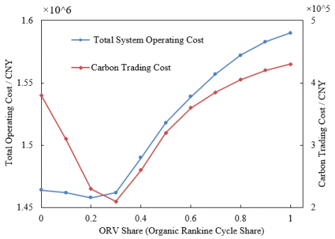
Figure 4. Impact of ORC capacity share on system cost and carbon trading performance
The study further explores how different installed capacities of Organic Rankine Cycle (ORC) waste heat power generation influence economic and carbon trading outcomes in a multi-regional system. As shown in Figure 4, increasing ORC capacity from 20% to 40% clearly reduces total system cost. This results from ORC’s ability to recover low-grade heat from industrial processes and CHP flue gas, improving thermodynamic efficiency and reducing reliance on costly electricity imports and natural gas. At the same time, the additional clean electricity displaces fossil-based generation, decreasing emissions and carbon trading costs. In some cases, increased ORC penetration even results in carbon revenue. However, when ORC capacity exceeds 50%, total cost rises again, indicating that the increase in capital and O&M costs outweighs marginal fuel and carbon savings. The results indicate an optimal ORC deployment level that balances thermodynamic efficiency gains against economic cost, providing quantitative guidance for planning low-carbon technologies in multi-regional systems.
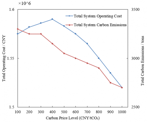
Figure 5. System-level impact of tiered carbon pricing on cost and carbon emissions
To quantify the system-level impacts and critical thresholds of tiered carbon pricing—a key policy variable—experiments were conducted. As shown in Figure 5, when carbon prices remain below ¥250/ton, system cost rises gradually while emissions decline slowly, indicating that low prices are insufficient to trigger operational changes. Once the first tier threshold is exceeded, emissions drop sharply and costs increase more rapidly, showing that carbon cost has become a dominant factor in dispatch decisions. The system responds by investing in or dispatching more low-/zero-carbon resources, raising cost but improving emissions. When prices exceed ¥500/ton (second threshold), emissions plateau while total cost spikes, as high trading costs or clean energy investment dominate. This suggests diminishing marginal abatement returns. The conclusion is that tiered carbon pricing effectively drives emission reductions, but economic cost rises nonlinearly. There exists a critical pricing window where carbon price adjustments yield the best economic-environmental balance, offering a key reference for fine-tuning carbon trading policy.
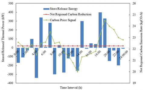
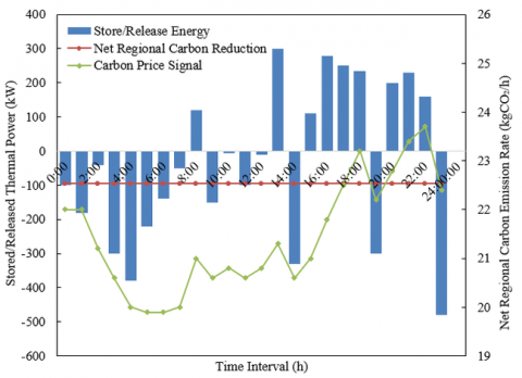
(a) Before optimization
(b) After optimization
Figure 6. Impact of multi-regional co-optimization on regional load and carbon reduction under carbon trading policy
Finally, the proposed framework’s effectiveness in responding to carbon pricing, improving system flexibility, and enhancing emission reductions is validated. As shown in Figure 6, prior to optimization, the system showed weak responsiveness to carbon price signals, and its charging/discharging behavior was poorly aligned with the spatiotemporal distribution of emissions. After coordinated optimization, energy storage strategies were highly synchronized with carbon price dynamics: heat was released during high-price periods to reduce reliance on costly, carbon-intensive external energy, and thermal energy was stored during low-price periods. This strategy significantly increased net regional carbon reduction during peak load hours and reduced total operating cost by lowering carbon expenditures, all while ensuring thermal comfort. The conclusion is that the proposed co-optimization framework effectively mobilizes distributed thermal inertia resources to participate in carbon markets. It transforms carbon price signals into actionable dispatch instructions, enabling significant improvements in both carbon performance and economic efficiency while maintaining energy service reliability.
This study presents a systematic investigation of a thermodynamics- and economics-based collaborative optimization model for multi-regional energy systems, developing a two-stage framework that integrates thermal network physical constraints with carbon trading economic mechanisms. The research includes the following key components: First, by conducting multi-regional thermal power flow analysis, determining initial flow rates, and minimizing total heat supply, the study establishes a thermodynamically efficient foundation for system operation and accurately quantifies energy transmission losses. Second, based on this physical groundwork, a collaborative optimization model is formulated to minimize both operating costs and carbon trading costs, enabling a system-wide analysis of multi-energy coupling among electricity, heat, and gas, as well as dynamic interregional energy exchanges.
The results clearly demonstrate that tiered carbon pricing policies outperform fixed carbon prices in stimulating deeper emission reductions. Specifically, within the carbon price range of ¥250-¥500 per ton, the system achieves an optimal balance between economic cost and environmental benefit. Furthermore, compared with independent regional operation, multi-regional coordinated optimization reduces total system cost by 16.4% and carbon emissions by 12.3%, underscoring the substantial value of breaking regional boundaries for spatial energy reallocation. Additionally, key low-carbon technologies such as P2G show significant advantages in enhancing renewable energy absorption and generating carbon trading revenue.
The primary academic contribution of this study lies in the proposal of a “physics-first, economics-driven” modeling paradigm, which offers a robust quantitative analysis tool and decision-support framework for the fine-tuned design and performance evaluation of carbon trading policies in complex multi-regional energy systems.
Nevertheless, some limitations remain. For example, the dynamic characteristics of thermal networks are simplified to ensure tractability; the model does not fully capture the strategic interactions among multiple market participants within the carbon market; and it assumes perfect market information and execution capability. Future research should focus on the development of fully coupled thermo-hydraulic dynamic models to enhance physical realism, the incorporation of game-theoretic or agent-based approaches to study multi-agent coordination under imperfect information, and the expansion of temporal scales to encompass both medium- and long-term infrastructure planning alongside short-term operations. These extensions will further refine the theoretical framework and practical roadmap for the low-carbon transition of multi-regional energy systems.
This paper was supported by Major Project of Fujian Social Science Fund Base: Research on the Valuation of Goodwill under the Background of "Dual Circulation" (Grant No.: FJ2022JDZ066).
[1] Balcilar, M., Özkan, O., Usman, O., Saint Akadırı, S., Zambrano-Monserrate, M.A. (2025). A global shift: How modern technologies are powering the energy transition in the face of climate change. Journal of Environmental Management, 384: 125610. https://doi.org/10.1016/j.jenvman.2025.125610
[2] Patil, G., Tiwari, C., Kavitkar, S., Makwana, R., et al. (2025). Optimising energy efficiency in India: A sustainable energy transition through the adoption of district cooling systems in Pune. Challenges in Sustainability, 13(1): 1-17. https://doi.org/10.56578/cis130101
[3] Mauludin, M.S., Khairudin, M., Asnawi, R., Prasetyo, S.D., Trisnoaji, Y., Rizkita, M.A., Arifin, Z., Rosli, M.A.M. (2025). Sustainable energy solutions in urban management: Carbon emissions and economic assessment of photovoltaic systems at electric vehicle stations in hybrid buildings. Challenges in Sustainability, 13(3): 377-397. https://doi.org/10.56578/cis130305
[4] Meng, X., Chen, M., Gu, A., Wu, X., Liu, B., Zhou, J., Mao, Z. (2022). China's hydrogen development strategy in the context of double carbon targets. Natural Gas Industry B, 9(6): 521-547. https://doi.org/10.1016/j.ngib.2022.11.004
[5] Shu, K., Guan, B., Zhuang, Z., Chen, J., et al. (2025). Reshaping the energy landscape: Explorations and strategic perspectives on hydrogen energy preparation, efficient storage, safe transportation and wide applications. International Journal of Hydrogen Energy, 97: 160-213. https://doi.org/10.1016/j.ijhydene.2024.11.110
[6] Singh, L.K., Mishra, G., Sharma, A.K., Gupta, A.K. (2021). A numerical study on thermal management of a lithium-ion battery module via forced-convective air cooling. International Journal of Refrigeration, 131: 218-234. https://doi.org/10.1016/j.ijrefrig.2021.07.031
[7] Li, G., Huang, G., Lin, Q., Cai, Y., Chen, Y., Zhang, X. (2012). Development of an interval multi-stage stochastic programming model for regional energy systems planning and GHG emission control under uncertainty. International Journal of Energy Research, 36(12): 1161-1174. https://doi.org/10.1002/er.1867
[8] Navidi, M., Moghaddas-Tafreshi, S.M., Alishvandi, A. M. (2021). A semi-decentralized framework for simultaneous expansion planning of privately owned multi-regional energy systems and sub-transmission grid. International Journal of Electrical Power & Energy Systems, 128: 106795. https://doi.org/10.1016/j.ijepes.2021.106795
[9] Miao, Z.J., Boamah, K.B., Long, X.L. (2020). Research on entropy generation strategy and its application in carbon trading market. Business Strategy and the Environment, 29(5): 1992-2000. https://doi.org/10.1002/bse.2483
[10] Knight, E.R.W. (2011). The economic geography of European carbon market trading. Journal of Economic Geography, 11(5): 817-841. https://doi.org/10.1093/jeg/lbq027
[11] Heidrich, M. (2024). General boundedness of energy exchange as alternative to the third law of thermodynamics. International Journal of Theoretical Physics, 63(11): 288. https://doi.org/10.1007/s10773-024-05831-4
[12] Hersh, M.A. (1998). Sustainable decision making and decision support systems. Computing & Control Engineering Journal, 9(6): 289-295. https://doi.org/10.1049/cce:19980610
[13] Zheng, W., Zou, B., Gu, J., Chen, J., Hou, J. (2024). Study on optimal allocation of energy storage in multi-regional integrated energy system considering stepped carbon trading. International Journal of Low-Carbon Technologies, 19: 551-558. https://doi.org/10.1093/ijlct/ctad111
[14] Song, X., Zhao, R., De, G., Wu, J., Shen, H., Tan, Z., Liu, J. (2020). A fuzzy-based multi-objective robust optimization model for a regional hybrid energy system considering uncertainty. Energy Science & Engineering, 8(4): 926-943. https://doi.org/10.1002/ese3.674
[15] Wang, J. X., Sun, Y. H., Siano, P. (2022). Integrated modeling of regional and park-level multi-heterogeneous energy systems. Energy Reports, 8: 3141-3155.
[16] Çomakli, K., Yüksel, B., Çomakli, Ö. (2004). Evaluation of energy and exergy losses in district heating network. Applied Thermal Engineering, 24(7): 1009-1017. https://doi.org/10.1016/j.applthermaleng.2003.11.014
[17] Zhang, X.M., Lu, F.F., Xue, D. (2022). Does China’s carbon emission trading policy improve regional energy efficiency?—An analysis based on quasi-experimental and policy spillover effects. Environmental Science and Pollution Research, 29(14): 21166-21183. https://doi.org/10.1007/s11356-021-17021-4
[18] Muñoz, J.C., Oliva, H.S., Sauma, E. (2024). Effect of combining carbon policies and price controls in cross-border trade of energy on renewable generation investments. Energy Journal, 45(1): 81-103. https://doi.org/10.5547/01956574.45.1.jmun
[19] Memari, A., Ahmad, R., Rahman, A.R.A., Jokar, M.R.A. (2018). An optimization study of a palm oil-based regional bio-energy supply chain under carbon pricing and trading policies. Clean Technologies and Environmental Policy, 20(1): 113-125.
[20] Bedogni, F., Rossi, E., Arfelli, F., Cespi, D., Passarini, F. (2025). Methodological challenges in wood carbon Accounting: A maritime flooring case study. Journal of Cleaner Production, 524: 146525. https://doi.org/10.1016/j.jclepro.2025.146525
[21] Dawley, S., MacKinnon, D., Cumbers, A., Pike, A. (2015). Policy activism and regional path creation: The promotion of offshore wind in North East England and Scotland. Cambridge Journal of Regions, Economy and Society, 8(2): 257-272. https://doi.org/10.1093/cjres/rsu036
[22] Boucekkine, R., Germain, M. (2009). The burden sharing of pollution abatement costs in multi-regional open economies. The BE Journal of Macroeconomics, 9(1): 34. https://doi.org/10.2202/1935-1690.1692