Tarek G. Emam
© 2022 IIETA. This article is published by IIETA and is licensed under the CC BY 4.0 license (http://creativecommons.org/licenses/by/4.0/).
OPEN ACCESS
In this work, nonlinear radiative flow over a vertical cylinder moving with a nonlinear velocity is presented. The mathematical model of the problem is formulated to include many parameters such as the thermal radiation parameter, the nonlinearity parameter, the Prandtl number, etc. Mathematica program is built to numerically solve the system of ordinary differential equations together with boundary conditions that is derived from the partial differential equations governing the fluid motion through using suitable similarity transformations. Numerical results obtained for the case of linear cylinder velocity are compared with analytical results obtained for the same case to validate the numerical method used in this work. Profiles of the fluid velocity and fluid temperatures are introduced and discussed to explore different parameters effects.
boundary layer flow, moving cylinder, nonlinear thermal radiation, nonlinear velocity, similarity solutions
It is known that the flow of Newtonian and Non-Newtonian fluids has many industrial applications, so a lot of authors have presented many studies in this field for the last few decades. We can find a lot of applications to the problem of our concern which is the study of the boundary layer flow over a moving cylinder. One can find such applications in wire drawings as well as in plastic and metallurgy industries.
Sakiadis [1] obtained a numerical solution to the problem of boundary layer flow over a moving cylinder using a similarity transformation. Rotte and Beek [2] have considered the heat transfer coefficients to a moving cylinder. Ganesan and Loganathan [3] have considered the problem of mass transfer effects and thermal radiation on flow of an incompressible viscous fluid past a moving vertical cylinder. Recently Ado-Eldahab and Salem [4] have considered a flow past a moving cylinder and taken into consideration the heat transfer of non-Newtonian power law fluid with chemical reaction and diffusion. Amkadni and Azzouzi [5] have given a study on the steady flow of an electrically conducting incompressible fluid over a moving vertical cylinder that is semi-infinite in the presence of a uniform transverse magnetic field. Due to its importance and valuable applications, the Study of hydrodynamic flow and the transfer of heat in a porous medium is very interesting. It has many applications in the process of controlling boundary layer flow such as the removal of heat from nuclear debris.
Elbashbeshy et al. [6] have studied the problem of boundary layer flow over a horizontal stretching that is embedded in a porous medium. They have studied the effects of heat transfer, thermal radiation, and suction/injection. An Analytic solution of the problem of flow of a micropolar fluid over moving cylinder taking into consideration axisymmetric stagnation flow has been introduced by Rehman et al. [7] and Rasheed et al. [8] have presented a study that gives a good view of the electrically conducting boundary layer flow of viscoelastic incompressible nanofluid which flows due to a moving linearly stretching surface. More recent papers of the subject of boundary layer flow over a cylinder can be found in the references [9-16].
In this paper we investigate the problem of heat and mass transfer and flow over a cylinder moving vertically with nonlinear velocity in the presence of nonlinear thermal radiation.
We consider an incompressible steady laminar flow over a cylinder that is moving with nonlinear velocity. We consider that the cylinder is semi-infinite with radius R. The fluid properties are constant. Axial coordinate x is measured along the axis of the cylinder. The radial coordinate r is measured normal to the axis of the cylinder. The two axes intersect at the origin. The external velocity is $u_e(x)=u_{\infty}\left(\frac{x}{l}\right)^n, u_{\infty}>0$.
The equations govern the model are:
$\frac{\partial(r v)}{\partial r}+\frac{\partial(r u)}{\partial x}=0$ (1)
$u \frac{\partial u}{\partial x}+v \frac{\partial u}{\partial r}=\frac{v}{r} \frac{\partial}{\partial r}\left(r \frac{\partial u}{\partial r}\right)+u_e \frac{d u_e}{d x}+\frac{v}{\mathrm{~K}_p}\left(u_e-u\right)$ (2)
$u \frac{\partial T}{\partial x}+v \frac{\partial T}{\partial r}=\frac{\alpha}{r}\left[\frac{\partial}{\partial r}\left(r \frac{\partial T}{\partial r}\right)-\frac{1}{\kappa} \frac{\partial}{\partial r}\left(r q_r\right)\right]$ (3)
Subject to the boundary conditions
$u(R, x)=u_w\left(\frac{x}{l}\right)^n$,
$v(R, x)=0, \lim _{r \rightarrow \infty} u(r, x)=u_{\infty}\left(\frac{x}{l}\right)^n$ (4)
$T(R, x)=T_w, T=T_{\infty}$, as $r \rightarrow \infty$ (5)
where, u and v stand for the velocity components along the x and r directions respectively, v is the kinematic viscosity, ρ is the fluid density, σ is the electrical conductivity of the fluid, l is the characteristic length, Kp is the porosity of the medium, α is the thermal diffusivity, κ is the thermal conductivity, and $q_r=\frac{-4 \sigma^*}{3 k^*} \frac{\partial T^4}{\partial r}$ is the radiation heat flux in the radial direction, where σ* is the Stefan-Boltzmann constant and k* is the Rosseland radiation absorptivity.
Defining a stream function $\psi$ as:
$r u=\frac{\partial \psi}{\partial r}, r v=-\frac{\partial \psi}{\partial x}$ (6)
where,
$\begin{aligned} \psi &=\sqrt{\frac{v R(n+1) u_{\infty}}{2}\left(\frac{x}{l}\right)^{n+1}} R f(\eta), \\ \eta &=\sqrt{\frac{u_{\infty}}{2 v R(n+1)}\left(\frac{x}{l}\right)^{n-1}} \frac{1}{R}\left(r^2-R^2\right) \end{aligned}$ (7)
where, f is the dimensionless stream function and η is the similarity variable which is also a dimentionless quantity.
The dimensionless temperature θ(η) is defined as:
$\theta(\eta)=\frac{T-T_{\infty}}{T_W-T_{\infty}}$ (8)
Substituting from Eqns. (6)-(8) into Eqns. (3)-(5) we get the following system of ordinary differential equations:
$\frac{2}{n+1}(\eta M+1) f^{\prime \prime \prime}(\eta)+\left(\frac{2 M}{n+1}+\frac{\epsilon(n+1)}{2} f(\eta)\right) f^{\prime \prime}(\eta)+n \epsilon\left(1-\left(f^{\prime}(\eta)\right)^2\right)-K\left(f^{\prime}(\eta)-1\right)=0$ (9)
$\frac{\varepsilon(n+1) P r}{4} f \theta^{\prime}+\frac{M}{(n+1)}\left(1+R d\left(1+\left(\theta_W-1\right) \theta\right)^3\right) \theta^{\prime}+\frac{M}{(n+1)}\left(\left\{1+R d\left(1+\left(\theta_W-1\right) \theta\right)^3\right\} C \theta^{\prime}\right)^{\prime}=0$ (10)
subject to the boundary conditions:
$f(0)=0, f^{\prime}(0)=\frac{u_W}{u_{\infty}}=a$,
$f^{\prime}(\infty)=1, \theta(0)=1, \quad \theta(\infty)=0$ (11)
where, $M=\sqrt{\frac{2 v(n+1)}{u_{\infty} R}\left(\frac{l}{x}\right)^{n-1}}, \epsilon=\frac{R}{l}$, the permeability parameter $K=\frac{v R}{K_p u_{\infty}}\left(\frac{l}{x}\right)^{n-1}, \operatorname{Pr}$ is the Prandtl number, the thermal radiation parameter $R d=\frac{16 \sigma^* T_{\infty}^3}{3 k^* \kappa}, \theta_W=\frac{T_W}{T_{\infty}}, C=$ $\frac{r^2}{M R^2}$.
Using the following assumptions:
$y_1=f, y_2=f^{\prime}, y_3=f^{\prime \prime}, y_4=\theta, y_5=\theta^{\prime}$
The system of Eqns. (9)-(11) is transformed into a system of first order differential equations as follows:
$y_1^{\prime}(\eta)=y_2(\eta)$ (12)
$y_2^{\prime}(\eta)=y_3(\eta)$ (13)
$\frac{2}{n+1}(\eta M+1) y_3^{\prime}(\eta)=-\left(\frac{2 M}{n+1}+\frac{\epsilon(n+1)}{2} y_1(\eta)\right) y_3(\eta)-n \epsilon\left(1-y_2^2(\eta)\right)+K\left(y_2(\eta)-1\right)$ (14)
$y_4^{\prime}(\eta)=y_5(\eta)$ (15)
$\frac{M}{(n+1)}\left(\left\{1+R d\left(1+\left(\theta_W-1\right) y_4(\eta)\right)^3\right\} C y_5(\eta)\right)^{\prime}=-\frac{M}{(n+1)}\left(1+R d\left(1+\left(\theta_W-1\right) y_4(\eta)\right)^3\right) y_5(\eta)-\frac{\epsilon(n+1) P r}{4} y_1(\eta) y_5(\eta)$ (16)
Subject to the initial conditions:
$y_1(0)=0, y_2(0)=a, y_3(0)=s, y_4(0)=1, y_5(0)=u$ (17)
The numerical values of the parameters are chosen in a suitable way. While s and u are priori unknown that are determined as a part of the solution.
The software Mathematica is used to solve the problem numerically through defining a function $F[s, u]:=$ NDSolve $[(12)-(17)]$. The unknown values s and u are found through solving the equations $y_2\left(\eta_{\max }\right)=1, y_4\left(\eta_{\max }\right)=0$. A reasonable start value is given to $\eta_{\max }$ and then increased to reach $\eta_{\max }$ for which the difference between two successive values of s and those of u are less than 107. Now the problem can be solved easily as an initial value problem using the function NDSolve. See references [16-18].
To validate the numerical method used in this paper we consider the velocity Eq. (9)
$(\eta M+1) f^{\prime \prime \prime}(\eta)+(M+\epsilon f(\eta)) f^{\prime \prime}(\eta)+\epsilon\left(1-\left(f^{\prime}(\eta)\right)^2\right)-K\left(f^{\prime}(\eta)-1\right)=0$ (18)
With the boundary conditions:
$f(0)=0, f^{\prime}(0)=\frac{u_W}{u_{\infty}}=a, f^{\prime}(\infty)=1$ (19)
where, $M=\sqrt{\frac{4 v}{u_{\infty} R}}$ and $K=\frac{v R}{K_p u_{\infty}}$.
The exact solution given in [17] is:
$f(\eta)=\eta+\frac{(a-1) M}{\epsilon}\left(1-e^{\frac{-\epsilon \eta}{M}}\right)$ (20)
where,
$K=\left(\frac{\epsilon}{M}\right)^2-\epsilon(a+2)$ (21)
Now we solve Eq. (18) with the initial conditions (19) numerically. The exact solutions and the numerical solutions are compared for some values of the considered parameters and exhibited in Table 1.
Table 1. Values of $f^{\prime \prime}(0)$ where $M=0.3, \epsilon=1$
|
$a$ |
Exact Soln. [17] |
Num. Soln. |
Error $\left|f^{\prime \prime}(0)-1\right|$ |
|
1.1 |
$-\frac{1}{3}$ |
-0.3333333 |
$2.722 \times 10^{-12}$ |
|
1.3 |
-1 |
-1.0000000 |
$1.529 \times 10^{-10}$ |
|
1.5 |
$-\frac{5}{3}$ |
-1.6666667 |
$8.240 \times 10^{-13}$ |
|
2 |
$-\frac{10}{3}$ |
-3.3333333 |
$7.450 \times 10^{-12}$ |
The numerical calculated value of $\left|f^{\prime \prime}(0)-1\right|$ is given in column 4 of Table 1. Exact values should be zeroes as $\eta_{\max } \rightarrow \infty$. So, one can assures that the numerical method used is valid.
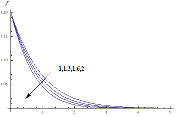
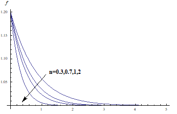
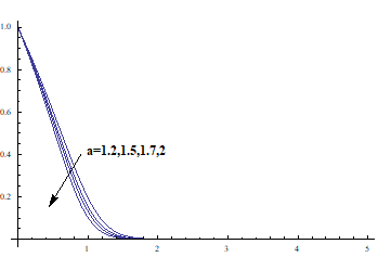
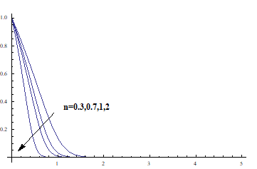
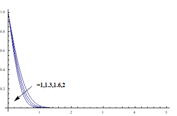
The solutions of the problem for different values of the considered parameters are given in this section. The variance of the fluid velocity $f^{\prime}(\eta)$ and the fluid temperature θ(η) with $\eta$ are plotted for different values of the parameters considered in the problem. As shown in Figures 1-5 the fluid velocity changes inversely with η till the fluid velocity takes the value of one which indicates the case of ambient fluid. Figure 1 shows how the parameter $\epsilon=\frac{R}{l}$ affects the fluid velocity. Decreasing $\epsilon=\frac{R}{l}$ results in increasing the fluid velocity. Such behavior is reasonable since the decrease of the cylinder radius R results in diminishing the cylinder surface area and consequently decreases the frictional force which in turn tend to increase the fluid velocity. The parameter n effect on the fluid velocity is exhibited in Figure 2. It is found that the increase of n results in decreasing the fluid velocity. To understand such behavior, we compare values of $f^{\prime \prime}(0)$ for different n values. The comparison shows that $f^{\prime \prime}(0)$ decreases with the increase of n which implies such effect shown in Figure 2. Figure 3 ensures that the increase of the initial velocity parameter $a$ will give rise to the fluid velocity.
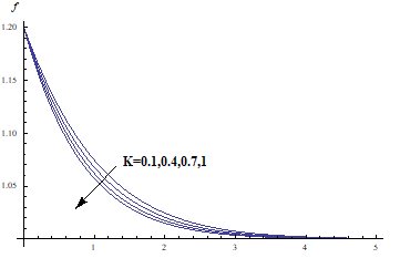
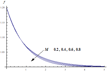
Table 2 shows that $-f^{\prime \prime}(0)$ increases with increasing $K$ which forces the fluid velocity to decrease as exhibited in Figure 4 . From Figure 5 one can find that the fluid velocity also decreases with the increase of $M$ since $-f^{\prime \prime}(0)$ increases with increasing $M$ as shown in Table 2 .
Figures 6-12 exhibit the variation of the fluid temperature similarity variable θ(η) which represents the difference between the fluid temperature and the ambient temperature with the similarity variable $\eta$.
The behavior of the graphs as expected shows that $\theta(\eta)$ decreases with the increase of $\eta$ damping to zero. The effects of different parameters considered in this article on $\theta(\eta)$ are also shown in figures that require physical interpretation. As the initial velocity parameter $a$ increases the fluid velocity increases and consequently the cooling rate increases also so $\theta(\eta)$ decrease which is shown clearly in Figure 6. Figure 7 exhibits the variation of the fluid temperature $\theta(\eta)$ with the parameter $n$. The increase of the parameter $n$ results in decreasing the fluid temperature. Since the increase of $n$ increases the surface heat flux $\left(-\theta^{\prime}(0)\right)$ as shown in Table 2.
Increasing the value of the parameter $\epsilon=\frac{R}{l}$ results in increasing the cylinder surface area which in turn tends to increase value of $-\theta^{\prime}(0)$ and so the value of $\theta(\eta)$ decrease as verified well in Figure 8.
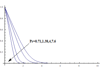
The effect of Prandtl number $P r$ on the fluid temperature $\theta(\eta)$ can be interpreted physically considering its definition $(\operatorname{Pr}=v / \alpha$ the ratio of momentum diffusivity (kinematic viscosity) to thermal diffusivity), the fluid thermal conductivity decreases with the increase of $\operatorname{Pr}$ and hence the surface heat flux (see Table 2) which in turn reduces the fluid temperature. Such behavior is detectable in Figure 9 .
Figure 10 shows the effect of the thermal radiation parameter $R d$ on the fluid temperature $\theta(\eta)$. To understand the variation of $\theta(\eta)$ with $R d$ we notice that the Rossland radiation absorptivity $k^*$ decreases with the increase of $R d$ and consequently the radiation heat flux $q_r=\frac{-4 \sigma^*}{3 k^*} \frac{\partial T^4}{\partial r}$ increases resulting in increasing the rate of radiative heat transferred to the fluid hence elevating the fluid temperature. As $\theta_W=\frac{T_W}{T_{\infty}}$ increases the wall temperature increases which in turn results in increasing the fluid temperature that can be noticed clearly upon investigating Figure 11.
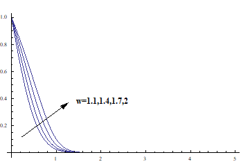
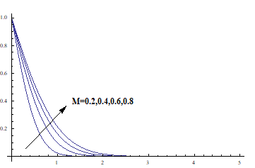
The variation of the fluid temperature $\theta(\eta)$ with the parameter $M$ is exhibited in Figure 12. From Table 2 one can notice that as $M$ increases the value of $-\theta^{\prime}(0)$ decreases; From the definition of the parameter $M=\sqrt{\frac{2 v(n+1)}{u_{\infty} R}\left(\frac{l}{x}\right)^{n-1}}$, one can notice that as $M$ increases the cylinder radius $R$ decreases which in turn results in diminishing the cylinder surface area that is lower the surface heat flux $-\theta^{\prime}(0)$ which leads to increasing the fluid temperature which is shown in Figure 12 .
Figure 1. Variation of the fluid velocity $f^{\prime}(\eta)$ with the parameter $\epsilon$, where $M=0.2, a=1.2, n=0.3, \theta_W=$ $1.1, K=0.4, \operatorname{Pr}=7.6, \mathrm{Rd}=1, C=2$
Figure 2. Variation of the fluid velocity $f^{\prime}(\eta)$ with the parameter $n$, where $M=0.2, a=1.2, \epsilon=1, \theta_W=2, K=1, \operatorname{Pr}=7.6, \mathrm{Rd}=1.2, C=2$
Figure 3. Variation of the fluid velocity $f^{\prime}(\eta)$ with the parameter $a$, where $M=0.2, n=0.3, \epsilon=1, \theta_W=2, K=1, \operatorname{Pr}=6.2, \mathrm{Rd}=1.2, C=2$
Figure 4. Variation of the fluid velocity $f^{\prime}(\eta)$ with the parameter $K$, where $M=0.2, n=0.3, \epsilon=1, \theta_W=2, a=1.2, \operatorname{Pr}=7.6, \operatorname{Rd}=1, C=2$
Figure 5. Variation of the fluid velocity $f^{\prime}(\eta)$ with the parameter $M$, where $K=0.4, n=0.3, \epsilon=1, \theta_W=1.1, a=1.2, \operatorname{Pr}=7.6, \operatorname{Rd}=1, C=2$
Figure 6. Variation of the fluid temperature $\theta(\eta)$ with the parameter $a$, where $M=0.2, n=0.3, \epsilon=1, \theta_W=2, \operatorname{Pr}=6.2, \mathrm{Rd}=1.2, C=2, K=1$
Figure 7. Variation of the fluid temperature $\theta(\eta)$ with the parameter $n$, where $M=0.2, a=1.2, \epsilon=1, \theta_W=2, a=1.2, \operatorname{Pr}=7.6, \mathrm{Rd}=1.2, C=2, K=1$
Figure 8. Variation of the fluid temperature $\theta(\eta)$ with the parameter $\epsilon$, where $M=0.2, a=1.2, n=0.3, \theta_W=1.1, a=1.2, \operatorname{Pr}=7.6, \mathrm{Rd}=1.2, C=2, K=0.4$
Figure 9. Variation of the fluid temperature $\theta(\eta)$ with the parameter $\operatorname{Pr}$, where $M=0.2, a=1.2, n=0.3, \theta_W=2, a=1.2, \epsilon=1, \operatorname{Rd}=1.2, C=2, K=1$
Figure 10. Variation of the fluid temperature $\theta(\eta)$ with the parameter $R d$, where $M=0.2, a=1.2, n=0.3, \theta_W=2, a=1.2, \epsilon=1, \operatorname{Pr}=7.6, C=2, K=1$
Figure 11. Variation of the fluid temperature $\theta(\eta)$ with the parameter $\theta_W$, where $M=0.2, a=1.2, n=0.3, R d=1, a=1.2, \epsilon=1, \operatorname{Pr}=7.6, C=2, K=1$
Figure 12. Variation of the fluid temperature $\theta(\eta)$ with the parameter $M$, where $\theta_W=1.1, a=1.2, n=0.3, R d=1, a=1.2, \epsilon=1, \operatorname{Pr}=7.6, C=2, K=0.4$
Table 2. Values of $-f^{\prime \prime}(0)$ and $-\theta^{\prime}(0)$ for various values of the considered parameters
|
n |
M |
$\epsilon$ |
K |
Pr |
Rd |
$\theta_w$ |
C |
$a$ |
$-f^{\prime \prime}(0)$ |
$-\theta^{\prime}(0)$ |
|
0.5 0.7 0.1 |
0.4 |
1.0 |
1.0 |
7.6 |
1.2 |
2.0 |
2.0 |
1.2 |
0. 294076 0.338875 0.405774 |
0.655995 0.717159 0.809287 |
|
0.5 |
0.2 0.4 0.6 |
1.0 |
1.0 |
7.6 |
1.2 |
2.0 |
2.0 |
1.2 |
0.284732 0.294076 0.303192 |
0.852847 0.655995 0.570127 |
|
0.5 |
0.4 |
1.0 1.5 2.0 |
1.0 |
7.6 |
1.2 |
2.0 |
2.0 |
1.2 |
0.294076 0.333143 0.367911 |
0.655995 0.760530 0.849012 |
|
0.5 |
0.4 |
1.0 |
0.4 0.7 1.0 |
7.6 |
1.2 |
2.0 |
2.0 |
1.2 |
0.259431 0.277313 0.294076 |
0.657275 0.656602 0.655995 |
|
0.5 |
0.4 |
1.0 |
1.0 |
0.7 4.0 7.6 |
1.2 |
2.0 |
2.0 |
1.2 |
0.294076 0.294076 0.294076 |
0.342671 0.528014 0.655995 |
|
0.5 |
0.4 |
1.0 |
1.0 |
7.6 |
1.2 1.7 2.0 |
2.0 |
2.0 |
1.2 |
0. 294076 0. 294076 0.294076 |
0. 655995 0.578398 0.546589 |
|
0.5 |
0.4 |
1.0 |
1.0 |
7.6 |
1.2 |
1.4 1.7 2.0 |
2.0 |
1.2 |
0. 294076 0. 294076 0. 294076 |
1.093853 0.829356 0. 655995 |
|
0.5 |
0.4 |
1.0 |
1.0 |
7.6 |
1.2 |
2.0 |
2.0 3.0 4.0 |
1.2 |
0. 294076 0. 294076 0. 294076 |
0. 655995 0.504565 0.420907 |
|
0.5 |
0.4 |
1.0 |
1.0 |
7.6 |
1.2 |
2.0 |
2.0 |
1.2 1.5 2.0 |
0. 294076 0.758729 1.592643 |
0. 655995 0.691506 0.747028 |
The problem of nonlinear radiative flow over a vertical cylinder moving with nonlinear velocity is studied. Mathematical model is introduced to formulate the problem including all parameters affecting the fluid velocity and temperature. The results obtained from the numerical method used to solve the problem was compared to those of exact solution in some special cases to show how accurate is the numerical method. The influences of the considered parameters are investigated and interpreted.
This work was funded by the University of Jeddah, Jeddah, Saudi Arabia, under grant No. (UJ-21-DR-115). The authors, therefore, acknowledge with thanks the University of Jeddah technical and financial support.
[1] Sakiadis, B.C. (1961). Boundary-layer behavior on continuous solid surfaces: II. The boundary layer on a continuous flat surface. AIChE Journal, 7(2): 221-225. https://doi.org/10.1002/aic.690070211
[2] Rotte, J.W., Beek, W.J. (1969). Some models for the calculation of heat transfer coefficients to a moving continuous cylinder. Chemical Engineering Science, 24(4): 705-716. https://doi.org/10.1016/0009-2509(69)80063-1
[3] Ganesan, P., Loganathan, P. (2002). Radiation and mass transfer effects on flow of an incompressible viscous fluid past a moving vertical cylinder. International Journal of Heat and Mass Transfer, 45(21): 4281-4288. https://doi.org/10.1016/S0017-9310(02)00140-0
[4] Abo-Eldahab, E.M., Salem, A.M. (2005). MHD Flow and heat transfer of non-Newtonian power law fluid with diffusion and chemical reaction on a moving cylinder. Heat and Mass Transfer, 41(8): 703-708. https://doi.org/10.1007/s00231-004-0592-7
[5] Amkadni, M., Azzouzi, A. (2006). On a similarity solution of MHD boundary layer flow over a moving vertical cylinder. Differential Equations and Nonlinear Mechanics, 2006: 1-9. https://doi.org/10.1155/DENM/2006/52765
[6] Elbashbeshy, Elsayed M.A., Emam, T.G., El-Azab, M.S., Abdelgaber, K.M. (2015). Effect of thermal radiation on flow, heat, and mass transfer of a nanofluid over a stretching horizontal cylinder embedded in a porous medium with suction/injection. J. Porous Media, 18(3): 215-229. https://doi.org/10.1615/JPorMedia.v18.i3.30
[7] Rehman, A., Iqbal, S., Raza, S.M. (2016). Axisymmetric stagnation flow of a Micropolar fluid in a moving cylinder: An analytical solution. Fluid Mechanics, 2(1): 1-7. https://doi.org/10.11648/j.fm.20160201.11
[8] Rasheed, H., Rehman, A., Sheikh, N., Iqbal, S. (2017). MHD boundary layer flow of nanofluid over a continuously moving stretching surface. Applied and Computational Mathematics, 6(6): 265-270. https://doi.org/10.11648/j.acm.20170606.15
[9] Loganathan, P., Eswari, B. (2017). Natural convective flow over moving vertical cylinder with temperature oscillations in the presence of porous medium. Global Journal of Pure and Applied Mathematics, 13(2): 839-855.
[10] Manjunatha, P.T., Gireesha, B.J., Prasannakumara, B.C. (2017). Effect of radiation on flow and heat transfer of MHD dusty fluid over a stretching cylinder embedded in a porous medium in presence of heat source. Int. J. Appl. Comput. Math, 3(1): 293-310. http://dx.doi.org/10.1007%2Fs40819-015-0107-x
[11] Abu Bakar, S., Arifin, N.M., Md Ali, F., Bachok, N., Nazar, R., Pop, I. (2018). A stability analysis on mixed convection boundary layer flow along a permeable vertical cylinder in a porous medium filled with a nanofluid and thermal radiation. Applied Sciences, 8(4): 483. https://doi.org/10.3390/app8040483
[12] Dalla Vedova, M., Alimhillaj, P. (2019). Novel fluid dynamic nonlinear numerical models of servovalves for aerospace. Int. J. Mech, 13: 39-51.
[13] Abdel-Wahed, M.S., El-Said, E.M. (2019). Magnetohydrodynamic flow and heat transfer over a moving cylinder in a nanofluid under convective boundary conditions and heat generation. Thermal Science, 23(6 Part B): 3785-3796. https://doi.org/10.2298/TSCI170911279A
[14] Mkhatshwa, M.P., Motsa, S.S., Ayano, M.S., Sibanda, P. (2020). MHD mixed convective nanofluid flow about a vertical slender cylinder using overlapping multi-domain spectral collocation approach. Case Studies in Thermal Engineering, 18: 1-12. https://doi.org/10.1016/j.csite.2020.100598
[15] Rahimi, H., Tang, X.N., Esmaeeli, Y., Li, M., Pourbakhtiar, A. (2020). Numerical simulation of flow around two side-by-side circular cylinders at high Reynolds number. International Journal of Heat and Technology, 38(1): 77-91. https://doi.org/10.18280/ijht.380109
[16] Elbashbeshy, Elsayed M.A., Emam, T.G., El-Azab, M.S., Abdelgaber, K.M. (2016). Slip effects on flow heat and mass transfer of nanofluid over stretching horizontal cylinder in the presence of suction/injection. Thermal Science, 20(6): 1813-1824. https://doi.org/10.2298/TSCI140512135E
[17] Emam, T.G. (2021). Boundary layer flow over a vertical cylinder embedded in a porous medium moving with non linear velocity. WSEAS Trans. Fluid Mech, 16: 32. https://doi.org/10.37394/232013.2021.16.4
[18] Emam, T.G., Elmaboud, Y.A. (2017). Three-dimensional magneto-hydrodynamic flow over an exponentially stretching surface. International Journal of Heat and Technology, 35(4): 987-996. https://doi.org/10.18280/ijht.350435