Johain J. Faraj | Fawizea M. Hussein | Ahmed J. Hamad*
© 2022 IIETA. This article is published by IIETA and is licensed under the CC BY 4.0 license (http://creativecommons.org/licenses/by/4.0/).
OPEN ACCESS
There are many approaches by which the heat exchanger can be modeled depending on how much information is available to start with. Grey-box model represents one of these approaches which is considered in the present study to modeling the unsteady operation heat exchanger. The available measurements of an unidentified heat exchanger integrated with a process involving oil circulation were statistically analyzed to extract the information that could aid in its identification. The proposed heat exchanger system included a hot oil stream coming from the thermal unit process and cooled by a cold-water circuit. The objective of this study is to develop a grey box model for the unspecified heat exchanger with a suitable nonlinear state-space structure and solved numerically using MATLAB-19 software and engineering equation solver (EES). Suitable parameters included oil and water inventories, heat addition, and conductance divisor factor are chosen to fully identify the heat exchanger from measured temperatures and flow rates. The parameters used to identify the oil process included the oil mass inventory within the process and the quantity of heat added. While for the heat exchanger; oil, water, and solid thermal masses were determined along with a conductance divisor to close its model. The results revealed that, comparing the model output with the measured data was satisfactory. The effect of 10% increment in the oil process heat as external excitation on a heat exchanger can only be controlled by water and oil flow rates and any fluctuation in inlet water temperature is insignificant and considered as a noise disturbance. An increment of 19% in the oil flowrate with unchanged water flowrate resulted in an increase in oil outlet temperature by about 4%. applying a noise of about ±10% on inlet water temperature to the system resulted in insignificant effects on the oil temperatures, and therefore it could be considered as uniform temperature. An effective control system to manage the heat exchanger and therefore the process can be designed according to the predictions of changing the water and oil flow rate responses.
heat exchanger, state space, unsteady performance, grey box, identification
Past decades have exhibited many oil-to-water heat exchanger steady performance studies to meet design loads [1-6]. Nevertheless, heat exchangers' good transient performance under serious working conditions has become mandatory in many circumstances, specifically for industries that require demanding conditions [7-9]. Satisfactory control of an industrial process requires a thorough knowledge of heat exchange transient responses in the whole system [10]. However, this is a complicated task because the transient responses will greatly fluctuate following the operational conditions [11, 12], and other system components' status [13].
Modeling of heat exchangers might improve the knowledge in this aspect. These models vary in their complexity, accuracy, and objectives [14]. Some documented models resorted to solving numerically the conservation differential equations [15-17]. These models require prior knowledge of the heat exchanger specification, arrangement, and configuration [18], in addition, they need extensive computational resources rendering them unsuitable for control purposes. Korzen and Taler [19] developed their model incorporating axial conduction effects which is simpler but still needs the finite volume method to solve the governing equations. They calculated the heat exchanger transient response to a sudden increase in water flow rate with a sudden decrease in air flow rate. An exhaustive work of Taler [20] collected theories for a range of heat exchanger types along with methods of solution in both steady and unsteady states. An emphasis was given to calculating wall temperature indicating its importance in the design and operational phases.
Apart from the aforementioned efforts, lumped parameters dynamic models are appealing since they require less computation [21] and they are easy to apply, an in-depth analysis could be found in ref. [22]. There are even attempts to find analytical solutions [23], nevertheless; they would be restricted. A more realistic approach was presented by Yao et al. [24] in which a linearized model was developed for an air to water heat exchanger used in HVAC systems. In addition, linearized models are excellent solutions when it comes to a dynamic model of systems containing multiple heat exchangers that coexist with other components [25].
The objective of this work is to lay out a grey box model for the unspecified heat exchanger with a suitable nonlinear state-space structure. Suitable parameters are to be chosen to fully identify the heat exchanger from measured temperatures and flow rates. It is expected that such a model will aid in the design and selection of a proper controller. The proposed model results are validated against available experimental data.
2.1 Heat exchanger system
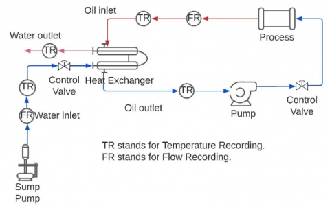
The heat exchanger process system was hypothetically separated into two parts, namely, the heat exchanger part and an abstract oil process part comprised of all other than the heat exchanger subprocesses. The proposed heat exchanger system included a hot oil stream coming from a thermal unit process which is cooled by a cold-water circuit. This system is equipped with the measuring devices and other required accessories as illustrated in Figure 1. The operating conditions of the heat exchanger is illustrated in the Table 1.
Figure 1. Schematic of heat exchanger integrated with a process
Table 1. Operating conditions of the heat exchanger
|
Property |
Specification |
|
Oil specific heat |
2 kJ/kg K |
|
Water specific heat |
4.17 kJ /kg K |
|
Process oil mass inventory |
4 kg |
|
Solid specific heat |
0.502 kJ/kg K |
|
Oil mass flow rate |
0.027 kg/s |
|
Water mass flow rate |
0.042 kg/s |
|
Process bulk oil temperature |
30℃ |
|
Heat exchanger solid temperature |
21℃ |
|
Exchanger bulk oil temperature |
25℃ |
|
Exchanger bulk water temperature |
18℃ |
|
Water inlet temperature |
16.5℃ |
|
Process heat addition |
0.5 kW |
2.2 Heat exchanger state-space model
There are three common approaches to modeling the heat exchanger depending on how much information is available to start with, namely, White, Black and Grey box models. White box models require detailed knowledge regarding heat exchanger specifications which may not always be available. On the other hand, black-box models offer simplicity and need only input-output data but at the expense of flexibility. Grey-box models exploit most of the above two models since they can be developed based on structures of white-box models like the state-space structure without prior knowledge of detailed specification. A single state variable Grey-box model was suggested for the oil part. The oil mass inventory is the oil confined in the process volume and results in some latency effects [24]:
$m_{o i l} C_{p o} \frac{d x_{1}}{d t}=Q+\dot{m}_{o} C_{p o} T_{i}-\dot{m}_{o} C_{p o} x_{1}$ (1)
or as a state-space model with two inputs.
$A=\left[-\frac{\dot{m}_{o}}{m_{o i l}}\right], \quad B=\left[\begin{array}{ll}\frac{\dot{m}_{o}}{m_{o i l}} & \frac{1}{m_{o i l} C_{p o}}\end{array}\right]$ (2)
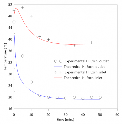
Figure 2 shows the output of this model with Ti taken from best fit to the measured oil inlet temperature. This left the model with two unknowns, i.e., oil mass inventory and external heat input, to be adjusted for the closest fit with outlet temperature. However, the theory couldn’t fit the measurement flawlessly, possible causes are either random noise or unaccounted for states.
Figure 2. Process oil input-output relationship
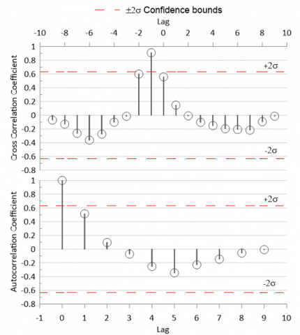
Figure 3 presents the error autocorrelation in which all correlations but at zero lag, are within the confidence bounds indicating probable random noise [26]. Thus, a need for a better and maybe higher-order model is recommended following the outcome of cross-correlation which indicates a possible correlation between the error and the input.
There are many methods by which the heat exchanger can be modeled depending on how much information is available to start with. In the current case, there are only measured temperatures at outlets and inlets without any specification for the process or the heat exchanger. Suitable parameters including oil and water inventories, heat addition, and conductance divisor factor (f) are chosen to fully identify the heat exchanger from measured temperatures and flow rates. Many published works are available on such cases ranging from artificial neural network (ANN) [27] to system identification [28] and other fitting methods [29]. The state-space method was selected in the current work with some unknown parameters left to be determined from measured data.
Figure 3. Error auto and cross correlations
The heat exchanger could be divided into 3 separate subsystems, water, oil, and solid material of the wall, assuming negligible axial conduction. Each one has its state, hence:
$C_{w} \frac{d T_{w}}{d x}=\dot{m}_{w} C_{p w} T_{w i}-\dot{m}_{w} C_{p w} T_{w e}-f U A\left(T_{w}-T_{S}\right)$ (3)
$C_{s} \frac{d T_{s}}{d x}=f U A\left(T_{w}-T_{s}\right)+(1-f) U A\left(T_{o}-T_{s}\right)$ (4)
$C_{o} \frac{d T_{o}}{d x}=\dot{m}_{o} C_{p o} T_{o i}-\dot{m}_{o} C_{p o} T_{o e}-(1-f) U A\left(T_{o}-T_{S}\right)$ (5)
where, Tw, To, and Ts are the bulk temperatures of the water, oil, and solid masses within the heat exchanger respectively. Cw, Co, and Cs are the corresponding heat capacitances, implicitly encompass water and oil inventory masses and solid material mass within the heat exchanger. With no other information available, a linear profile is assumed for temperature variation throughout the heat exchanger. These equations were used to find the equilibrium values and then rearranged into a linearized space state model as follows:
$\left[\begin{array}{l}\dot{x}_{1} \\ \dot{x}_{2} \\ \dot{x}_{3} \\ \dot{x}_{4}\end{array}\right]$$=\left[\begin{array}{cccc}-a_{11} & 0 & 0 & a_{11} \\ 0 & a_{22} & a_{23} & 0 \\ 0 & a_{32} & a_{33} & a_{34} \\ a_{41} & 0 & a_{43} & a_{44}\end{array}\right]\left[\begin{array}{l}x_{1} \\ x_{2} \\ x_{3} \\ x_{4}\end{array}\right]$$+\left[\begin{array}{cccc}0 & \frac{1}{m_{o} C_{p o}} & 0 & 2 \frac{\left(-x_{1}^{e}+x_{4}^{e}\right)}{m_{o}} \\ 2 \frac{\dot{m}_{w}{ }^{e} C_{p w}}{C_{w}} & 0 & 2 \frac{C_{p w}}{C_{w}}\left(-x_{2}^{e}+T_{w i}^{e}\right) & 0 \\ 0 & 0 & 0 & 0 \\ 0 & 0 & 0 & 2 \frac{C_{p o}}{C_{o}}\left(x_{1}^{e}-x_{4}^{e}\right)\end{array}\right]\left[\begin{array}{c}T_{w i} \\ Q \\ \dot{m}_{w} \\ \dot{m}_{o}\end{array}\right]$ (6)
where:
x1: bulk oil temperature perturbation within the process.
x2: bulk water temperature perturbation within the heat exchanger.
x3: bulk solid temperature perturbation within the heat exchanger.
x4: bulk oil temperature perturbation within the heat exchanger.
$\mathrm{a}_{11}=2 \frac{\dot{m}_{o}}{m_{o i l}}$
$\mathrm{a}_{22}=-\frac{1}{C_{w}}\left(2 \dot{m}_{w} C_{p w}+f U A\right)$
$\mathrm{a}_{23}=\frac{f U A}{C_{w}}$
$\mathrm{a}_{32}=\frac{f U A}{C_{S}}$
$\mathrm{a}_{33}=-\frac{U A}{C_{S}}$
$\mathrm{a}_{34}=\frac{(1-f) U A}{C_{S}}$
$\mathrm{a}_{41}=\frac{2 \dot{m}_{o} C_{p o}}{C_{o}}$
$\mathbf{a}_{43}=\frac{(1-f) U A}{C_{o}}$
$\mathrm{a}_{44}=-\frac{1}{C_{o}}\left(2 \dot{m}_{o} C_{p o}+(1-f) U A\right)$
The superscript "e" denotes equilibrium conditions. From the steady measurements of the heat exchanger, UA was estimated to be around 0.2 kW/K. This UA should be divided between oil and water sides, by which (1-f) UA goes to the oil side and f UA to the water side. The value of conductance divisor factor (f) is between 0 and 1 and adjusted according to experimental data.
The fluctuation in the process heat is to be alleviated by controlling oil and water flow rates. The figure of merit here is the bulk oil temperature (x1) since it is an indication of the temperature in the process itself.
Although, Twi is being handled with the input matrix, but it is more like a disturbance than a controlled input. The cooling water supply is a very large reservoir and assumed of constant temperature, however; measurements show some fluctuations. A sample of more than 140 water inlet temperature observations were taken. The mean of the sample inlet water temperature was 16.5℃ with a sample standard deviation of 1.93℃.
The justification of selecting the above-mentioned inputs and states is discussed in regard to field measurements. Water flow rate changes throughout plant operation from 100 to about 250 L/h. Since the heat exchanger is integrated with the process utilizing the oil, this should reflect on the return oil temperature which is the inlet to the heat exchanger. This relation is governed, however; by other than heat exchanger plant systems which may have more influencing factors. Two immanent effects are initial rate at which oil temperature decreased and the final steady temperature.
The solution methodology of the heat exchanger model considered in the present research work is based on choosing a suitable structure in the grey-box model. The structure should incorporate all inputs, outputs, and operational parameters into an appropriate mathematical formulation. In this work, the non-linear state-space structure was implemented followed by an optimization process using MATLAB identification toolbox capabilities for non-linear grey box models to estimate all unknown parameters. This process closes the model rendering it ready for performance prediction. The complete model is then coded in a MATLAB program for the calculation of the output variable against a varying range of inputs.
The Model unknown parameters were adjusted for the minimum discrepancy between model output and experimental data as illustrated in Figure 4 which show the comparison between theoretical and experimental oil temperatures. Although the trend is almost similar, there are some deviations of about 6% between theoretical and experimental data.
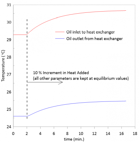
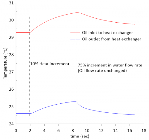
Figure 5 shows the effect of 10% increment in the process heat on inlet and outlet oil temperatures. From system control point of view, the external excitation is the heat added to oil when it passes through the process. Water inlet temperature is uncontrollable and any fluctuation that may occur is considered as a noise disturbance.
To compensate for these changes, either water or oil or both streams mass flow rate should be readjusted to keep the process stable. For a step increase in heat delivered to the oil, the system responded with nearly steady rise in oil temperature as depicted in Figure 5.
An attempt to counteract this effect by increasing the water flow rate is illustrated in Figure 6 which shows the effect of increment in the water flow rate on oil inlet and outlet temperatures. As a consequence, exit oil temperature is brought near its initial value. The exit oil should be brought below the initial value to convey excess heat without elevating the process temperature. An increase of 75% in water flow rate could not fulfill this requirement because of the heat exchanger capacity limitations.
Figure 4. Comparison between theoretical and experimental oil temperatures
Figure 5. Effect of increment in the process heat on oil temperature
Figure 6. Effect of increment in water flow rate on oil temperature
Figure 7 shows the effect of increment in oil flow rate on oil inlet and outlet temperatures. Increasing the oil flow rate is not very successful since it accompanied by an increase in oil outlet temperature which in turn has a negative impact on process oil temperature.
It can be observed in this figure that, a 19% increment in the oil flowrate with unchanged water flowrate has resulted in an increase in oil outlet temperature by about 4%. The impact of inlet water temperature noise on the heat exchanger inlet and outlet oil temperatures is shown in Figure 8. It can be concluded that applying a noise of about ±10% on inlet water temperature to the system resulted in a little response in oil temperature. It has almost insignificant effects on the oil temperatures, and hence; the noise in temperature could be neglected and consider it as uniform to save computation resources.
Figure 7. Effect of increment in oil flow rate on oil temperature
Figure 8. Impact of inlet water temperature noise on oil temperatures
The suggested grey box model represents a reasonable approach in identifying a heat exchanger integrated with the oil process and could be used to implement an appropriate controller for managing process temperature. In summary, some points could be drawn from the results:
The authors express their sincere appreciation to the workers in the computer center and workshop of the Engineering Technical College, Middle Technical University for supporting us to achieve this study.
|
A |
state matrix |
|
B |
input matrix |
|
C |
heat capacity, kW. K-1 |
|
Cp |
specific heat, kJ. kg-1. K-1 |
|
f |
conductance divisor factor (0 – 1) |
|
moil |
oil mass inventory within the process |
|
$\dot{m}$ |
mass flow rate, kg. s -1 |
|
Q |
external heat input, W |
|
UA |
overall heat transfer coefficient kW. K-1 |
|
T |
temperature, K |
|
Subscripts |
|
|
e |
exit |
|
i |
inlet |
|
o |
oil |
|
s |
solid material |
|
w |
water |
[1] Dubey, V.V.P., Verma, R.R., Verma, P.S., Srivastava, A.K. (2014). Steady state thermal analysis of shell and tube type heat exchanger to demonstrate the heat transfer capabilities of various thermal materials using Ansys. Global Journal of Researches in Engineering, 14(4): 25-30.
[2] Ranong, C.N., Roetzel, W. (2002). Steady-state and transient behavior of two heat exchangers coupled by a circulating flow stream. International Journal of Thermal Sciences, 41(11): 1029-1043. https://doi.org/10.1080/01457630590959449
[3] Karthik, S., Tawfiq A., Al Abdul, Q., Al Saikhan, Al Abdulwahed, A.A. (2016). Design of a hot oil heat exchanger. International journal of Applied Engineering Research, 11(20): 10102-10124.
[4] Egeregor, D. (2008). Numerical simulation of heat transfer and pressure drop in plate heat exchangers using FLUENT as a CFD Tool. MSc. Thesis, Blekinge Institute of Technology, Karlskrona, Sweden.
[5] Silaipillayarputhur, K., Al‐mughanam, T. (2021). Performance of pure crossflow heat exchanger in sensible heat transfer application. Energies, 14(17). https://doi.org/10.3390/en14175489
[6] Chyhryn, S. (2019). Modelling and analysis of plate heat exchangers for flexible district heating systems. Energies, 12(21). https://doi.org/10.3390/en12214141
[7] Popov, I.A., Gortyshov, Y.F., Olimpiev, V.V. (2012). Industrial applications of heat transfer enhancement: The modern state of the problem (a Review). Thermal Engineering, 59(1): 1-12. https://doi.org/10.1134/S0040601512010119
[8] Gao, T., Sammakia, B., Geer, J. (2017). Transient effectiveness methods for the dynamic characterization of heat exchangers. In. Tech. https://doi.org/10.5772/67334
[9] Yousef, B., Abdelhafid, B., Sakina, Z., et al. (2017). Numerical and experimental investigation on the transient behavior of an earth air heat exchanger in continuous operation mode. International Journal of Heat and Technology, 35(2): 279-288. http://dx.doi.org/10.18280/ijht.350208
[10] Marchal, P.C., Ortega, J.G., García. J.G. (2018). Advances in Industrial Control: Production Planning, Modeling and Control of Food Industry Processes. Book, Springer International Publishing, [Online]. https://www.springer.com/gp/authors-editors/journal-author/journal-author-help.
[11] Fotowat, S., Askar, S., Fartaj, A. (2021). A transient response comparison of a conventional and a meso heat exchanger under mass flow and temperature step changes. Journal of Fluid Flow, Heat and Mass Transfer, 8: 199-216. https://doi.org/10.11159/jffhmt.2021.022
[12] Mai, T.H., Chitou, N., Padet, J. (1999). Heat exchanger effectiveness in unsteady state. EPJ Applied Physics, 8(1): 71-75. https://doi.org/10.1051/epjap:1999231
[13] Bequette, B.W., Russo, L.P. (2003). Chemical process design, simulation, optimization, and operation. in Encyclopedia of Physical Science and Technology, Elsevier, pp. 751-766. https://doi.org/10.1016/b0-12-227410-5/00100-9
[14] Bonilla, J., Alberto, D.C., Margarita, R.G., Roca, L., Valenzuela, L. (2017). Study on shell-and-tube heat exchanger models with different degree of complexity for process simulation and control design. Applied Thermal Engineering, 124: 1425-1440.
[15] Kilic, M., Ullah, A. (2021). Numerical investigation of effect of different parameter on heat transfer for a crossflow heat exchanger by using nanofluids. Journal of Thermal Engineering, 7(14): 1980-1989. http://dx.doi.org/10.18186/thermal.1051287
[16] Sai, S.K., Nandhanagopal, G.R., Yarrapathruni, V.H.R. (2021). Modelling and parametric analysis of wire finned coiled tube heat exchanger in a small J-T refrigerator. International Journal of Heat and Technology, 39(3): 913-918.
[17] Ravindra, K.P., Manindra, B., Subba, R.J., Appa, R.K. (2021). Computational analysis of conventional and helical finned shell and tube heat exchanger using ANSYS-CFD. International Journal of Heat and Technology, 39(6): 1755-1762. https://doi.org/10.18280/ijht.390608
[18] Sharma, S., Sharma, S., Singh, M., Singh, P., Singh, R., Maharana, S., Khalilpoor, N., Issakhov, A. (2021). Computational fluid dynamics analysis of flow patterns, pressure drop, and heat transfer coefficient in staggered and inline shell-tube heat exchangers. Mathematical Problems in Engineering, 2021, ID 6645128. https://doi.org/10.1155/2021/6645128
[19] Korzeń, A., Taler, D. (2017). Mathematical modeling of unsteady response of plate and fin heat exchanger to sudden change in liquid flow rate. E3S Web of Conferences, 14(1): 1023. https://doi.org/10.1051/e3sconf/20171401023
[20] Taler, D. (2019). Numerical modelling and experimental testing of heat exchangers. Springer Professional. https://doi.org/10.1007/978-3-319-91128-1
[21] Gentsch, M., King, R. (2021). A low-order dynamic model of counterflow heat exchangers for the purpose of monitoring transient and steady-state operating phases. Chemical Engineering Science, 235: 116241. https://doi.org/10.1016/j.ces.2020.116241
[22] Wilfried, R., Xing, L., Dezhen, C. (2019). Design and Operation of Heat Exchangers and Their Networks. Academic Press; 1st edition, 2019.
[23] Ansari, M.R., Mortazavi, V. (2007). Transient response of a co-current heat exchanger to an inlet temperature variation with time using an analytical and numerical solution. Numerical Heat Transfer; Part A: Applications, 52(1): 71-85. https://doi.org/10.1080/10407780601114981
[24] Yao, Y., Huang, M., Mo, J., Dai, S. (2013). State-space model for transient behavior of water-to-air surface heat exchanger. International Journal of Heat and Mass Transfer, 64: 173-192. https://doi.org/10.1016/j.ijheatmasstransfer.2013.04.037
[25] Sun, X., Liu, L., Zhuang, Y., Zhang, L., Du, J. (2020). Heat exchanger network synthesis integrated with compression-absorption cascade refrigeration system. Processes, 8(2): 210. https://doi.org/10.3390/pr8020210
[26] Box, G.E.P., Jenkins, G.M., Reinsel, G.C. (1994). Time Series Analysis: Forecasting and Control, 3rd ed. Englewood Cliffs, NJ: Prentice Hall.
[27] Benyekhlef, A., Mohammedi, B., Hassani, D., Hanini, S. (2021). Application of artificial neural network (ANN-MLP) for the prediction of fouling resistance in heat exchanger to MgO-water and CuO-water nanofluids. Water Science & Technology, 84(3): 538. https://doi.org/10.2166/wst.2021.253
[28] Hanif, O., Deshpande, N.G., Chatterjee, M. (2021). Identification and control of a heat exchanger. International symposium of Asian control association on intelligent robotics and industrial automation (IRIA). pp. 259-264. https://doi.org/10.1109/IRIA53009.2021.9588708
[29] Gupta, S., Gupta, R., Padhee, S. (2018). Parametric system identification and robust controller design for liquid-liquid heat exchanger system. IET Control Theory and Applications, 12(10). https://doi.org/10.1049/iet-cta.2017.1128