Andres A. Sánchez-Escalona* | Yanán Camaraza-Medina | Ever Góngora-Leyva | Yoalbys Retirado Mediaceja
© 2022 IIETA. This article is published by IIETA and is licensed under the CC BY 4.0 license (http://creativecommons.org/licenses/by/4.0/).
OPEN ACCESS
A new methodology was established in order to determine forced convective heat transfer film coefficients, for single-phase non-laminar flow inside tubes. A comprehensive Nusselt number correlation was proposed, which is able to evolve into three different functional forms derived from the analogies among momentum, heat and mass transfer, as proposed by Reynolds-Colburn, Prandtl and von-Kármán. Parameters estimation was carried out by applying Genetic Algorithms, using the maximum relative error as the objective function. The methodology was verified against six synthetic data sets, with the independent variables within the ranges 2.4·103 ≤ Re < 5.0·106, 0.715 ≤ Pr ≤ 84101, 0.255 < μ/μw < 5.077, and the dependent variable Nu calculated by applying the Dittus-Boelter, Sieder & Tate, Petukhov, Gnielinski, von-Kármán and Camaraza-Medina correlations. Functional forms and initial equations coefficients were properly approximated. Comparison of calculated Nusselt numbers versus the reference values resulted in Pearson correlations higher than 99.85 %. Uncertainty related to the film coefficient calculation was found acceptable in all the cases. Proposed approach not only overcomes the simplicity of power-type correlations, but also avoids the drawbacks of non-linear regression methods and, unlike symbolic regression, it creates mathematical expressions starting from a previous theoretical-physical background instead of finding random correlations. Further stages of this study would focus on evaluating a wider range of μ/μw and validating the methodology with experimental data.
analogies, boundary layer, convection, genetic algorithms, heat exchanger
The design, sizing and rating of heat exchangers requires reliable calculation of the overall heat transfer coefficient. Conventional literature reference values or empirical expressions quantifying local convective heat transfer coefficients are assumed, when the overall coefficient cannot be experimentally determined by measuring both fluids mass flowrates, inlet and outlet temperatures [1, 2]. In such cases, the use of inappropriate or inexact correlations may result in under- or over-sizing of the equipment, as well as incorrect estimation of the fouling factor and thermal system efficiency. Therefore, besides being a crucial parameter that favors decision-making within the industrial field, accurate determination of convective film coefficients is a challenging problem with applications in several branches of science and engineering [3-5].
There are several empirical methods for experimental determination of convective heat transfer coefficients. In this respect, the simplest ones apply Newton’s Cooling Law to obtain local coefficients from measurement of the heat flux, the heat transfer area, and the fluid and surface temperatures [6, 7]. The main drawback of this direct method relies on the difficulty to install thermocouples on heat exchanger plates or tube walls when they are inaccessible [8, 9].
Wilson [10] found an alternative to previous limitation, recommending separation of the overall thermal resistance into the inside convective thermal resistance and the remaining thermal resistances participating in the heat transfer process. This methodology, referenced in the specialized literature as the Wilson Plot method, is based on measurements of both fluids mass flowrates, inlet and outlet temperatures, over the studied heat exchanger. Despite the original Wilson Plot method was improved by Briggs and Young [11], Khartabil et al. [12], Shah [13], Khartabil and Christensen [14], Rose [15], van-Rooyen et al. [16], among other researchers, these studies assume a simple power law relationship between the surface heat transfer coefficient and the fluid flowrate, which is often not valid and generates large error margins. Generally, monomial power-type correlations do not provide good approximations over a broad range of experimental data [17-19]. Inaccuracies are largely influenced by inability of equations based on Reynolds analogy to describe the momentum and heat transfer phenomena that take place into the boundary layer, as it assumed that eddy diffusivity of heat is exactly analogous to the eddy diffusivity of momentum, besides no difference between viscous and turbulent eddies [20].
Non-linear regression methods overcome the restrictions associated with power-type correlations and the number of parameters to be estimated. Styrylska and Lechowska [21] analyzed the Wilson Plot method as a least squares adjustment problem based on the Newton gradient, rather than a linearized regression problem. Moreover, Flores et al. [3] used the Nelder-Mead approach to estimate the convective heat transfer coefficient in a helical condenser integrated to a thermal transformer. Another branch of investigations took advantage of current computational capabilities and numerical regression techniques, therefore using the Levemberg-Marquardt method for simultaneous determination of both-sides convective heat transfer coefficients, as studied by Taler [22-24] and Rainieri et al. [25]. Although representing an advantage over linear methods, multi-modal minimization problems based on gradients calculation do not guarantee that the global minimum is reached and are dependent of the initial point. They can only operate efficiently if realistic initial values are selected, which is virtually impossible where large number of unknowns are evaluated and little prior knowledge is available about the expected results [17, 26].
The growth of artificial intelligence tools contributed to the development of different solution methods. In this context, both Artificial Neural Networks (ANN) and Genetic Algorithms (GA) have been used to propose new correlations. Although ANN were only used for specific applications, they were found appropriate to simulate complex-flow convection heat transfer processes, like those happening on complex-geometry surfaces, streams on the transition zone, and uncommon chemicals experimenting phase changes [27-32]. In spite of the contributions introduced by the previous-mentioned studies, the use of ANN on this field enclose the following disadvantages: most of the data have been gathered through the direct experimental method (based on Newton’s Cooling Law); it is practically impossible to obtain the correlation explicit equation and, if formulated, it would be too complicated for practical purposes; the friction factor has not been previously considered as a predictor variable; and the traditional method provides insufficient information about the influence of independent variables on model response.
According to Mehdipour et al. [33], GA are simpler and faster than ANN. In addition to their significant performance in optimization problems, several authors have recognized their capability as an alternative curve-fitting and parameter estimation method. GA can operate with irregular non-differentiable functions, are not initial-point dependent, and explore a large portion of the design space thus unlikely converging to a local optimum. While some studies were aimed to determine forced convective heat transfer correlations for special applications [26, 34-37], a few others focused on correlations being applicable for heat exchange equipment [33, 38-40]. Although the use of GA for film coefficients determination have obvious advantages over other procedures, application of the simple method in accessed papers is yet limited by the following: the correlation functional form needs to be assumed a priori; only four unknowns are determined in most studies; and the practice of using power-type expressions still persist. Even though the mathematical function relating the Nusselt number to the remaining dimensionless parameters is generally selected on the basis of simplicity, compactness and common usage, it cannot be just justified according to these first principles. This issue demands special attention, as it can significantly limit the estimates accuracy [29, 41].
In order to overcome the aforementioned problem, another group of researchers put into practice symbolic regression methods. Unlike the parametric regression, this approach allows to determine both the correlation functional form as well as the constants in it. To achieve this, Genetic Programming (GP) algorithms were used, which are an extension of the GA. However, the expressions reported in the reviewed literature [41-46] have different functional forms and it is difficult to associate a physical meaning or theoretical support to the regression functions. Other drawbacks from applying the method are: complexity of obtained correlations; extensive expressions that limit a broader use in practical applications; high computational cost; poor generalization; and random results since there is no consistency among responses from different runs.
A previous analysis of the state of the art reveals that none of the preceding methods simultaneously consider the following premises: Correlation parameters not limited to the typical three unknowns of the power-type equations, effectiveness of the method to be independent of the initial-point selection, and evolution of the correlation functional form to be allowed for best fitting to the experimental data, without occurring deliberately and deprived of a physical sense. Taking these gaps into consideration, this research objective was to propose a new methodology for determination of forced convective heat transfer film coefficients by simulating evolution of Nusselt equation by means of GA, applicable to single-phase non-laminar flow inside tubes.
Following are main contributions declared for this study:
The remaining part of this paper is organized as follows: Section 2 describes materials and methods, focusing on the methodology for film coefficients determination and data sets collection; Section 3 shows the most relevant results, providing a quantitative and qualitative assessment of correlations obtained for each data set; and Section 4 refers to the main conclusions arrived by this study.
2.1 Film coefficients determination methodology
Parameters estimation to determine the functional form and coefficients of the Nusselt correlations was carried out by means of GA, due to the advantages of this stochastic search and optimization technique [47, 48]. Selected fitness function was the maximum relative error, calculated from the reference and theoretical Nusselt values, denoted as Nu and Nu' respectively.
The dependent variable reference values (Nu) were synthetically obtained, using acknowledged correlations to calculate the Nusselt number under forced convection, single-phase non-laminar internal flow conditions. Chosen independent variables were the Reynolds number (Re), the Prandtl number (Pr), the fluid dynamic viscosity at its mean temperature (μ), the viscosity at wall temperature (μw), as well as a binary variable which defines whether the heat exchange is related to a cooling or a heating process (P).
On the other hand, the dependent variable theoretical values (Nu') were calculated from a novel, generalized equation, which have the ability to evolve into three different functional forms derived from the Reynolds-Colburn, Prandtl and von-Kármán analogies. Coefficients of the correlation were determined, in each case, by decoding the genotype of the best fit individual, after running the GA. Given the random nature of this technique, each approximation process was run five times.
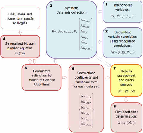
Effectiveness of the proposed methodology was tested against six different synthetic data sets, in which the independent variables values are repeated, but those of the dependent parameter are varied because of using different correlations to calculate the Nusselt number. Besides performing a mathematical-similitude comparison between the initial and the obtained Nusselt equations, Pearson’s correlation coefficient and a few error indexes were used to assess the quality of the results (Figure 1).
Figure 1. Methodology flowchart
Film coefficients were calculated from Eq. (1), once obtained the Nusselt number correlation with the best fitting to the experimental data [1, 20].
$h=\frac{k}{d}\cdot Nu'$ (1)
where: h – film coefficient or local convective heat transfer coefficient, W/(m2·K); Nu' – Nusselt number theoretical value; k – fluid thermal conductivity, W/(m·K); d – tube inside diameter (or equivalent diameter for other duct geometries), m.
2.2 Synthetic data sets collection
2.2.1 Variables selection
Mostly, equations describing the Nusselt number for forced convection under single-phase non-laminar flow conditions, inside tubes, satisfy Eq. (2) [49-51].
$Nu=\phi \left( Re;\text{ }Pr;\text{ }d\text{; }L\text{; }f;\text{ }{{J}_{\mu }} \right)$ (2)
where: Nu – Nusselt number; Re – Reynolds number; Pr – Prandtl number; L – tube length, m; f – Darcy-Weisbach friction factor; Jμ – viscosity correction factor, commonly calculated through Eq. (3):
${{J}_{\mu }}={{\left( \mu /{{\mu }_{w}} \right)}^{m}}$ (3)
where: μ – dynamic viscosity at fluid bulk temperature, Pa·s; μw – dynamic viscosity at wall temperature, Pa·s; m – correction factor equation exponent. Mondal and Field [52] recommended m = 0.254 for cooling and m = 0.087 for heating, based on a classical theoretical analysis of the thermal boundary layer. Their proposal constitutes an update of the correction factor exponents provided by Sieder and Tate [53] and Petukhov [54].
Simplification of Eq. (2) can be performed by taking the following into consideration:
Based on previous assumptions, Eq. (4) was deduced to define the predictive (independent) and response (dependent) variables that were used to validate the model:
$Nu=\phi \left( Re;\text{ }Pr;\text{ }\mu ;\text{ }{{\mu }_{w}};\text{ cooling or heating} \right)$ (4)
2.2.2 Independent variables values
Thermo-physical properties of eight common chemicals were used to generate the synthetic data sets, by considering working temperature ranges that are usual at industrial thermal processes. In this way, reference values for Prandtl number (Pr) and fluid dynamic viscosity (μ) were taken from the specialized literature [49, 55] to create a record of 80 data points (Table 1).
This initial data log was combined with eight values of the Reynolds number variable (Re), as shown on the column vector denoted by Eq. (5), therefore obtaining a 640 points database. Considered range for the Reynolds number would allow evaluation of flow regimes varying from the transition region to the fully turbulent zone.
$\begin{align} & Re=\left[ 2.4\cdot {{10}^{3}};\text{ 5}\text{.0}\cdot {{10}^{3}};\text{ }{{10}^{4}};\text{ 5}\text{.0}\cdot {{10}^{4}};\text{ }{{10}^{5}}; \right. \\ & \text{ }\left. 5.0\cdot {{10}^{5}};\text{ }{{10}^{6}};\text{ }5.0\cdot {{10}^{6}} \right] \\\end{align}$ (5)
The fluid dynamic viscosity evaluated at wall temperature (μw) was related to a binary variable that defines the heat transfer mode, using P = 1 for cooling and P = 0 for heating. On the first case, μw was obtained by considering the fluid viscosity at a temperature lower than the bulk temperature. On the second one, μw was considered at the higher temperature. Both situations are summarized in Eq. (6), which makes a distinction of the wall surface temperature according to the chemical compound under analysis.
Table 1. Initial data log
|
Fluid |
Temp. 1 (K) |
Data points |
Pr 1 |
μ 1 (Pa·s) |
|
Methanol |
293.15 343.15 |
6 |
4.655 7.414 |
3.146·10-4 5.857·10-4 |
|
Isobutane |
173.15 373.15 |
9 |
3.256 12.650 |
6.483·10-5 9.305·10-4 |
|
Glycerin |
273.15 313.15 |
9 |
2697 84101 |
3.073·10-1 10.490 |
|
Engine oil (unused) |
273.15 433.15 |
9 |
84 46636 |
4.500·10-3 3.814 |
|
Carbon dioxide 2 |
323.15 2273.15 |
10 |
0.744 0.882 |
1.612·10-5 7.322·10-5 |
|
Hydrogen 2 |
323.15 2273.15 |
10 |
0.715 1.172 |
9.430·10-6 3.690·10-5 |
|
Steam 2 |
373.15 973.15 |
10 |
0.981 0.880 |
1.200·10-5 3.650·10-5 |
|
Water 3 |
273.15 573.15 |
17 |
13.700 0.905 |
1.790·10-3 8.590·10-5 |
|
Total |
173.15 2273.15 |
80 |
0.715 84101 |
9.430·10-6 10.490 |
Notes: 1 Minimum and maximum values of the range are shown.
2 Properties at atmospheric pressure (101.3 kPa).
3 Properties at saturation pressure.
${{\mu }_{w}}=f({{T}_{w}})=f\left( \left\{ \begin{align} & {{T}_{\infty }}\pm 5,\text{ if Glycerin } \\ & {{T}_{\infty }}\pm 10,\text{ if Methanol, Isobutane } \\ & {{T}_{\infty }}\pm 20,\text{ if Oil, Steam} \\ & {{T}_{\infty }}\pm 50,\text{ if C}{{\text{O}}_{\text{2}}}\text{, }{{\text{H}}_{\text{2}}}\text{, Water} \\\end{align} \right. \right)$ (6)
where: Tw – average wall temperature, K; T∞ – fluid bulk temperature, K; subtraction operator (–) for cooling and addition operator (+) for heating.
2.2.3 Dependent variable values
In order to appraise the proposed solution effectiveness during approximation of different data sets, six expressions were used to calculate the Nusselt number, whilst using the same independent variables data. Selection of the following correlations relies on number of citations, recurrent publications within academic books, as well as recognition from the international scientific community:
$N{{u}_{D-B}}=0.023\cdot R{{e}^{0.8}}\cdot P{{r}^{m}}$ (7)
where: m = 0.3 for cooling, and m = 0.4 for heating.
$N{{u}_{S\And T}}=0.027\cdot R{{e}^{0.8}}\cdot P{{r}^{1/3}}\cdot {{\left( \mu /{{\mu }_{w}} \right)}^{0.14}}$ (8)
$N{{u}_{Pt}}=\frac{\left( f/8 \right)\cdot Re\cdot Pr}{C+12.7\sqrt{f/8}\cdot \left( P{{r}^{2/3}}-1 \right)}\cdot {{\left( \mu /{{\mu }_{w}} \right)}^{m}}$ (9)
$C=1.07+\frac{900}{Re}-\frac{0.63}{1+10\cdot Pr}$ (9a)
where: m = 0.25 for cooling, m = 0.11 for heating, and m = 0 for uniform heat flux or gasses.
$N{{u}_{Gn}}=\frac{\left( f/8 \right)\cdot (Re-1000)\cdot Pr}{1+12.7\sqrt{f/8}\cdot \left( P{{r}^{2/3}}-1 \right)}\cdot {{\left( \mu /{{\mu }_{w}} \right)}^{m}}$ (10)
$N{{u}_{vK}}=\frac{0.0288\cdot R{{e}^{0.8}}\cdot Pr}{1+0.849\cdot R{{e}^{-0,1}}\cdot \left[ \left( Pr-1 \right)+\ln \left( \frac{5\text{ }Pr+1}{6} \right) \right]}$ (11)
$N{{u}_{C-M}}=\frac{\left( Re-{{10}^{D}} \right)\cdot Pr}{A\cdot {{B}^{2}}-C\cdot B\cdot \left( 1-P{{r}^{2/3}} \right)}\cdot {{\left( \mu /{{\mu }_{w}} \right)}^{m}}$ (12)
$A=\left\{ \begin{matrix} 75.440,\text{ if 2400 }Re\text{ 1}{{\text{0}}^{4}}\text{ } \\ 91.415,\text{ if 1}{{\text{0}}^{4}}\text{ }\le \text{ }Re\text{ } \\\end{matrix} \right.$ (12a)
$B=\log \left( \frac{R{{e}^{0.56}}}{3.196} \right)$ (12b)
$C=\left\{ \begin{matrix} 104.00,\text{ if 2400 }Re\text{ 1}{{\text{0}}^{4}}\text{ } \\ 116.74,\text{ if 1}{{\text{0}}^{4}}\text{ }\le \text{ }Re\text{ } \\\end{matrix} \right.$ (12c)
$D=\left\{ \begin{matrix} \begin{align} & -0.027\cdot {{(logRe)}^{2}}\text{+0}\text{.2}\cdot logRe+2.63,\text{ } \\ & \text{ if 2400 }Re\text{ 1}{{\text{0}}^{4}}\text{ } \\\end{align} \\ 0,\text{ if 1}{{\text{0}}^{4}}\text{ }\le \text{ }Re\text{ } \\\end{matrix} \right.$ (12d)
2.3 Correlation coefficients and functional form determination
2.3.1 Parameters estimation by means of Genetic Algorithms
A methodology based on GA was developed during the present investigation, using MATLAB® R2013a scripts to determine coefficients and functional form of the convective heat transfer Nusselt correlations. The objective function and other implemented equations are described on sections 2.3.2 and 2.3.3. Options and parameters related to the algorithm configuration are detailed below (Table 2).
Table 2. GA configuration
|
Category |
Parameter |
Value |
|
Population |
Population size |
1000 |
|
Fitness scaling |
Scaling function |
Rank |
|
Selection |
Selection function |
Stochastic uniform |
|
Reproduction |
Elite count |
2 |
|
|
Crossover fraction |
0.5 |
|
Mutation |
Mutation function |
Constraint dependent |
|
Crossover |
Crossover function |
Scattered |
|
Migration |
Fraction |
0.2 |
|
|
Interval |
20 |
|
Constraints |
Initial penalty |
10 |
|
|
Penalty factor |
100 |
|
Stop criteria |
Generations |
200 |
|
|
Time limit |
∞ |
|
|
Fitness limit |
-∞ |
|
|
Stall generations |
50 |
|
|
Stall time limit |
∞ |
|
|
Function tolerance |
10-12 |
|
|
Nonlinear constraint tolerance |
10-6 |
GA are a global iterative search technique inspired by the Darwinian principle of natural selection. The problem is solved by imitating the mechanisms of species evolution through optimization strategies based on three basic operators: selection, crossover and mutation. As a concept, a group of individuals (population) changes from generation to generation, undergoing a process in which the stronger ones are likely to be the winners in a competing environment. Its mathematical analogy consists on a function to minimize (or maximize) and a search space for the desired solution, so that each point within this space corresponds to a value of the objective function and the target is to find the point that optimizes this function. In this way, the algorithm searches for the best optimum possible solution to the given problem [47, 62].
2.3.2 Objective function (or fitness function)
It was determined that the correlation that best describes the dependent variable reference values is the one that minimizes the Nusselt number maximum relative error, as expressed in Eq. (13).
$\underset{\mathbf{X},\mathbf{Y}}{\mathop{\arg \min }}\,\left[ \max \left( \sum\limits_{i=1}^{n}{\frac{\left| N{{u}_{i}}-Nu{{'}_{i}}(\mathbf{X},\mathbf{Y}) \right|}{N{{u}_{i}}}} \right) \right]$ (13)
where: Nu – dependent variable reference value; Nu' – dependent variable theoretical value calculated as function of vectors $\mathbf{X}$ and $\mathbf{Y}$; n – number of data points. Vector $\mathbf{X}$ includes the parameters to be estimated by the GA, while $\mathbf{Y}$ is comprised by the values of the independent variables (Re, Pr, μ, μw and P).
2.3.3 Comprehensive Nusselt number equation
Several researchers have studied the analogies among momentum, heat and mass transfer for turbulent flow. This theory is based on description of the fluid flow through the continuity equations, the Navier-Stokes equations and boundary conditions, hence decoupling the momentum and energy expressions under constant property assumption. The experimental evidences and similarity among both dimensionless expressions indicates that solution of one of these processes conveys to mathematical resolution of the other analogous phenomenon [20, 63].
The link between heat and momentum transfer for turbulent flows in straight round pipes was firstly developed by Reynolds in 1874. His postulates were subsequently improved by Chilton and Colburn in 1934, by extending its applicability to fluids with Pr ≠ 1 and Sc ≠ 1 (Sc stands for the Schmidt number). This empirical adjustment to the original approach is often referenced as Reynolds-Colburn analogy. The initial model was also modified by Prandtl in 1928, and later by von-Kármán in 1939, who pronounced new concepts about the flow-patterns distribution within the boundary layer. Since then, mentioned analogies have been used and enhanced by several researchers, consequently proving their convenience for physical explanation and a more accurate representation of the forced convection heat transfer mechanisms [20, 63, 64].
Unification of the main concepts, besides the need of integrating resultant convective heat transfer correlations, have encouraged the authors of this paper to formulate a comprehensive Nusselt number expression, without making distinction between the Reynolds-Colburn, Prandtl or von-Kármán analogies, as shown on Eq. (14).
Previous expression, used to determine the dependent variable theoretical value, is considered the main contribution of this study. It involves eight parameters (b1, b2, d1, d2, c1, c2, c3 y c4) that define the coefficients and functional form of the Nusselt number correlation. In turn, they are related to the vector (X) that characterizes the GA genotype (Figure 2).
$N u^{\prime}=\frac{c_{1} \cdot\left(\frac{f}{8}\right)^{b_{1} \cdot b_{2}} \cdot\left(e^{c_{2}^{\left(1-b_{1} \cdot b_{2}\right)}}-b_{1} \cdot b_{2} \cdot c_{3}\right) \cdot P r^{d_{1}^{\left(1-b_{1}\right)}}}{\left\{1+c_{4} \cdot R e^{-0.1\left(1-b_{2}\right)} \quad \cdot \quad \left(\frac{f}{8}\right)^{0.5 b_{2}} \quad \left[\left(P r^{d_{2}}-1\right)+\left(1-b_{2}\right) \cdot \ln \left(\frac{5 P r+1} {6} \right)\right]\right\}^{ \quad \quad b_{1}}}$$\cdot J_{\mu}$ (14)
Figure 2. Genetic Algorithm decoding
The first two parameters only admit binary values, according to Eq. (14a) and Eq. (14b). They were conceived to identify the momentum, heat and mass transfer analogy that best describes the experimental data:
$b_{1}=\left\{\begin{array}{l}0, \text { if Reynolds analogy, } \\ 1, \text { if superior analogies (Prandtl or von-Kárán). }\end{array}\right.$ (14a)
$b_{2}= \begin{cases}0, & \text { if von-Kármán analogy } \\ 1, & \text { if Prandtl analogy }\end{cases}$ (14b)
The second set of parameters, as defined by Eq. (14c) and Eq. (14d), acquires discrete values associated with the Prandtl number exponent:
${{d}_{1}}=\left\{ 1/3;\text{ }2/5 \right\}$ (14c)
${{d}_{2}}=\left\{ 2/3;\text{ 1} \right\}$ (14d)
Remaining parameters are curve-fitting correlation coefficients, which were intended to admit real values within the intervals described by Eq. (14e) to Eq. (14h). They are influenced by geometry of the heat transfer surface, flow characteristics, the heat exchanger operating conditions, and fouling differential effect [62, 65]. Exponent c2 also depends on the Prandtl number [19].
$\text{0 }{{c}_{1}}\le \text{ 1}$ (14e)
$\text{0 }{{c}_{2}}\le \text{ 1}$ (14f)
$\text{0 }\le \text{ }{{c}_{3}}\text{ }\le \text{ 1500}$ (14g)
$\text{0 }{{c}_{4}}\le \text{ 20}$ (14h)
3.1 Approximation of correlations derived from Reynolds-Colburn analogy
Parameter estimation results are shown below for the two data sets generated with the Dittus-Boelter and Sieder & Tate correlations, respectively (Tables 3-4).
Table 3. Parameters estimation using “Dittus-Boelter” data set
|
Variables |
|
Algorithm runs |
||||
|
|
1 |
2 |
3 |
4 |
5 |
|
|
Computed coefficients |
b1 |
0 |
0 |
0 |
0 |
0 |
|
b2 |
0 |
1 |
0 |
1 |
1 |
|
|
d1 |
2/5 |
2/5 |
2/5 |
2/5 |
2/5 |
|
|
d2 |
2/3 |
2/3 |
2/3 |
1 |
2/3 |
|
|
c1 |
0.023 |
0.023 |
0.023 |
0.023 |
0.023 |
|
|
c2 |
0.8 |
0.8 |
0.8 |
0.8 |
0.8 |
|
|
c3 |
358.5 |
99 |
805.5 |
1282.5 |
252 |
|
|
c4 |
19.82 |
10.66 |
13.26 |
10.26 |
6.66 |
|
|
Algorithm performance |
f obj |
0.00004 |
0.00005 |
0.00005 |
0.00006 |
0.00008 |
|
i |
104 |
52 |
101 |
58 |
78 |
|
|
sc 1 |
2 |
2 |
2 |
2 |
2 |
|
Notes: 1 Stop criteria:
1. Maximum number of generations exceeded;
2. Average change in the fitness value less than options.
Table 4. Parameters estimation using “Sieder & Tate” data set
|
Variables |
|
Algorithm runs |
||||
|
|
1 |
2 |
3 |
4 |
5 |
|
|
Computed coefficients |
b1 |
0 |
0 |
0 |
0 |
0 |
|
b2 |
0 |
0 |
1 |
1 |
1 |
|
|
d1 |
1/3 |
1/3 |
1/3 |
1/3 |
1/3 |
|
|
d2 |
2/3 |
2/3 |
1 |
2/3 |
2/3 |
|
|
c1 |
0.027 |
0.027 |
0.027 |
0.027 |
0.027 |
|
|
c2 |
0.8 |
0.8 |
0.8 |
0.8 |
0.8 |
|
|
c3 |
502.5 |
334.5 |
1270.5 |
195.0 |
277.5 |
|
|
c4 |
8.74 |
1.26 |
1.20 |
16.24 |
11.9 |
|
|
Algorithm performance |
f obj |
0.0014 |
0.0014 |
0.0014 |
0.0014 |
0.0014 |
|
i |
72 |
96 |
109 |
92 |
79 |
|
|
sc |
2 |
2 |
2 |
2 |
2 |
|
where: f obj – objective function value once the algorithm stops; i – number of iterations.
The algorithm conveniently identifies the functional form and quickly determines the exact coefficients of the Nusselt equation (Dittus-Boelter and Sieder & Tate cases). When substituting computed coefficients into Eq. (14), obtained correlations matches the initial ones selected to produce the synthetic data sets (Table 5).
Consequently, a strong linear association between the two variables was observed when comparing the Nusselt number calculated values (Nu') against the reference ones (Nu), which was confirmed by Pearson correlation coefficients equal to the unity. Determined error indexes are negligible, and mainly attributed to rounding inaccuracies (Table 6).
Table 5. Approximation of correlations derived from Reynolds-Colburn analogy
|
Target |
Obtained correlation |
|
Eq. (7) |
$Nu{{'}_{D-B}}=0.023\cdot R{{e}^{0.8}}\cdot P{{r}^{0.4}}$ |
|
Eq. (8) |
$Nu{{'}_{S\And T}}=0.027\cdot R{{e}^{0.8}}\cdot P{{r}^{1/3}}\cdot {{J}_{\mu }}$ |
Table 6. Calculated correlation and error indexes
|
Parameters |
Data set |
|
|
Dittus-Boelter |
Sieder & Tate |
|
|
R |
1 |
1 |
|
e ave |
4.9233·10-4 |
1.1047·10-2 |
|
e max |
3.7298·10-3 |
0.2300 |
|
E ave |
0.0185 |
0.5685 |
|
E max |
0.4271 |
37.7351 |
where: R – Pearson correlation coefficient; e ave – mean relative error, %; e max – maximum relative error, %; E ave – mean absolute error; E max – maximum absolute error.
3.2 Approximation of correlations derived from Prandtl analogy
The methodology was also tested for equations derived from Prandtl analogy. In this context, parameter estimation results are shown below for data sets produced through Petukhov and Gnielinski correlations (Tables 7-8).
The functional form was correctly approximated for these two cases, and similar coefficients were obtained as compared to those from Petukhov and Gnielinski expressions. Therefore, when substituting calculated coefficients into Eq. (14), similar correlations were obtained (Table 9). Note that when computed parameters diverge between different model runs, the statistical mode values were used to formulate the Nusselt number correlation.
Comparison of the Nusselt number calculated values (Nu') against the synthetic data (Nu) resulted in a remarkable degree of association between the two variables and low error indexes (Table 10).
The higher deviations were obtained during approximation of Petukhov correlation, since the comprehensive Nusselt number equation tries replacement of C (parameter included in the denominator of the original correlation) by using a fixed value. As observed in Eq. (9a) this is not a constant parameter, but depends on the Reynolds and Prandtl dimensionless numbers. Despite this peculiarity low relative errors were reached (below 3.4 %), firstly because C → 1 for most of the Re and Pr evaluated values, and secondly due to the Eq. (14) adaptability potential, which compensates existing deviations by adjusting other parameters considered in their functional form (c1, c3 and c4).
Table 7. Parameters estimation using “Petukhov” data set
|
Variables |
|
Algorithm runs |
||||
|
|
1 |
2 |
3 |
4 |
5 |
|
|
Computed coefficients |
b1 |
1 |
1 |
1 |
1 |
1 |
|
b2 |
1 |
1 |
1 |
1 |
1 |
|
|
d1 |
2/5 |
1/3 |
2/5 |
1/3 |
2/5 |
|
|
d2 |
2/3 |
2/3 |
2/3 |
2/3 |
2/3 |
|
|
c1 |
0.991 |
0.991 |
0.991 |
0.991 |
0.991 |
|
|
c2 |
0.725 |
0.654 |
0.832 |
0.914 |
0.460 |
|
|
c3 |
565.5 |
565.5 |
567.0 |
565.5 |
565.5 |
|
|
c4 |
12.3 |
12.3 |
12.3 |
12.3 |
12.3 |
|
|
Algorithm performance |
f obj |
0.0334 |
0.0334 |
0.0334 |
0.0334 |
0.0334 |
|
i |
118 |
108 |
185 |
73 |
100 |
|
|
sc |
2 |
2 |
2 |
2 |
2 |
|
Table 8. Parameters estimation using “Gnielinski” data set
|
Variables |
|
Algorithm runs |
||||
|
|
1 |
2 |
3 |
4 |
5 |
|
|
Computed coefficients |
b1 |
1 |
1 |
1 |
1 |
1 |
|
b2 |
1 |
1 |
1 |
1 |
1 |
|
|
d1 |
2/5 |
2/5 |
1/3 |
2/5 |
1/3 |
|
|
d2 |
2/3 |
2/3 |
2/3 |
2/3 |
2/3 |
|
|
c1 |
1.000 |
0.999 |
0.999 |
0.999 |
0.999 |
|
|
c2 |
0.363 |
0.125 |
0.268 |
0.377 |
0.899 |
|
|
c3 |
1000.5 |
1000.5 |
1000.5 |
1000.5 |
1000.5 |
|
|
c4 |
12.72 |
12.70 |
12.70 |
12.70 |
12.70 |
|
|
Algorithm performance |
f obj |
0.0014 |
0.0014 |
0.0014 |
0.0014 |
0.0014 |
|
i |
112 |
98 |
71 |
87 |
86 |
|
|
sc |
2 |
2 |
2 |
2 |
2 |
|
Table 9. Approximation of correlations derived from Prandtl analogy
|
Target |
Obtained correlation |
|
Eq. (9) |
$Nu{{'}_{Pt}}=\frac{0.991\cdot \left( \frac{f}{8} \right)\cdot (Re-565.5)\cdot Pr}{1+12.3\sqrt{\frac{f}{8}}\cdot \left( P{{r}^{2/3}}-1 \right)}\cdot {{J}_{\mu }}$ |
|
Eq. (10) |
$Nu{{'}_{Gn}}=\frac{0.999\cdot \left( \frac{f}{8} \right)\cdot (Re-1000.5)\cdot Pr}{1+12.7\sqrt{\frac{f}{8}}\cdot \left( P{{r}^{2/3}}-1 \right)}\cdot {{J}_{\mu }}$ |
Table 10. Calculated correlation and error indexes
|
Parameters |
Data set |
|
|
Petukhov |
Gnielinski |
|
|
R |
0.99981 |
1 |
|
e ave |
2.0200 |
9.9306·10-2 |
|
e max |
3.3800 |
0.1600 |
|
E ave |
503.7323 |
18.4271 |
|
E max |
1.2149·104 |
548.2273 |
3.3 Approximation of correlations derived from von-Kármán analogy
Parameter estimation results are also presented for the data set generated using von-Kármán correlation (Table 11).
The original equation functional form was properly identified through proposed solution method in four out of the five runs that were carried out. However, the second run converged to a local minimum of the objective function that corresponds to the Reynolds-Colburn analogy. As a result, when substituting computed coefficients into Eq. (14), two different correlations were obtained: one similar to von-Kármán expression, in a more precise and developed form; plus another one close to the Dittus-Boelter equation, but approximating in a lesser extent the Nusselt number reference values (Table 12).
Since the GA initial population is randomly generated, in a few occasions the parameter estimation results did not match. In such cases it is advisable to perform several runs, then select the solution that provides the more accurate results. Although not being part of the scope of this study, increasing the population size would avoid premature convergence of the objective function towards a local optimum.
Despite acceptable goodness of fit was determined when comparing the Nusselt number calculated values (Nu') versus the synthetic ones (Nu), the higher performance was achieved through the functional form associated to the von-Kármán analogy. Low error indexes were obtained by means of equation$Nu{{'}_{vK.1}}$, contrasting with average deviations beyond 10 % for equation $Nu{{'}_{vK.2}}$ which is linked to the Reynolds-Colburn analogy. Because of the higher errors, this last expression was rejected as a solution (Table 13).
Table 11. Parameters estimation using “von-Kármán” data set
|
Variables |
|
Algorithm runs |
||||
|
|
1 |
2 |
3 |
4 |
5 |
|
|
Computed coefficients |
b1 |
1 |
0 |
1 |
1 |
1 |
|
b2 |
0 |
1 |
0 |
0 |
0 |
|
|
d1 |
1/3 |
2/5 |
2/5 |
1/3 |
2/5 |
|
|
d2 |
1 |
2/3 |
1 |
1 |
1 |
|
|
c1 |
0.029 |
0.018 |
0.030 |
0.030 |
0.029 |
|
|
c2 |
0.801 |
0.837 |
0.801 |
0.800 |
0.801 |
|
|
c3 |
508.5 |
61.5 |
324.0 |
1083.0 |
1216.5 |
|
|
c4 |
0.80 |
13.46 |
0.82 |
0.82 |
0.80 |
|
|
Algorithm performance |
f obj |
0.0785 |
0.2650 |
0.0785 |
0.0784 |
0.0785 |
|
i |
78 |
84 |
100 |
93 |
80 |
|
|
sc |
2 |
2 |
2 |
2 |
2 |
|
Table 12. Approximation of correlations derived from von-Kármán analogy
|
Target |
Obtained correlations |
|
Eq. (11) |
$Nu{{'}_{vK.\text{1}}}=\frac{0.029\cdot R{{e}^{0.801}}\cdot Pr}{1+0.8\cdot R{{e}^{-0.1}}\cdot \left[ \left( Pr-1 \right)+\ln \left( \frac{5\text{ }Pr+1}{6} \right) \right]}$ |
|
|
$Nu{{'}_{vK.2}}=0.018\cdot R{{e}^{0.837}}\cdot P{{r}^{0.4}}$ |
Table 13. Calculated correlation and error indexes
|
Parameters |
Functional form |
|
|
von-Kármán |
Reynolds-Colburn |
|
|
R |
0.99851 |
0.98698 |
|
e ave |
3.2600 |
10.9700 |
|
e max |
8.5500 |
28.1900 |
|
E ave |
75.6148 |
274.4738 |
|
E max |
2.2988·103 |
7.0395·103 |
3.4 Approximation of novel correlations
Robustness and stability of the proposed solution method was finally verified versus the synthetic data set generated by using the Camaraza-Medina correlation (Table 14). Despite the authors selected the Prandtl analogy to deduce their expression, and adjusted the correlation coefficients based on a wider range of experimental data, their functional form does not exactly reproduce the structure of other correlations derived from this analogy.
Considering that no adaptation of the comprehensive equation matches Camaraza-Medina’s mathematical form, the implemented methodology has identified different correlations to approximate the target expression (Table 15).
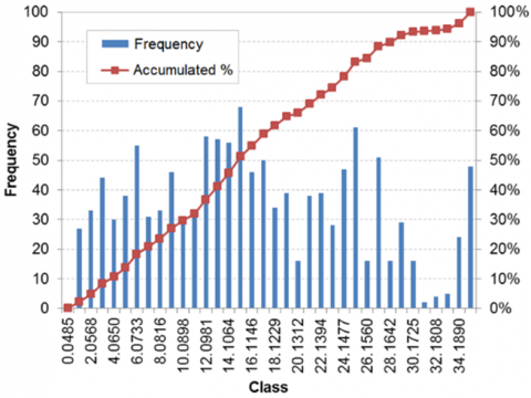
When evaluating the Pearson's correlation coefficient to compare the Nusselt number estimated values $\left(N u^{\prime}\right)$ versus the reference data $(N u)$, it was determined that the functional form based on von-Kármán analogy $\left(N u_{C-M .1}^{\prime}\right)$ provides the strongest association between the variables, followed in descending order by the equations consistent with Prandtl $\left(N u_{C-M .2}^{\prime}\right)$ and Reynolds-Colburn $\left(N u_{C-M .3}^{\prime}\right)$ analogies. Considering the above, besides calculated error indexes (Table 16), it is recommended to use the first expression $\left(N u_{C-M .1}^{\prime}\right)$ for approximation of Camaraza-Medina correlation. It provides relative deviations equal or lower than $20 \%$ in $65.95 \%$ of the evaluated data points (Figure 3).
Although the functional form based on von-Kármán analogy proved to be the most accurate, maximum deviation values are considered high in all three cases. This is attributed to the fact that the proposed methodology tries a single-equation approximation of Camaraza-Medina correlation, which, as observed in Eq. (12), was adjusted for two pre-defined ranges of the Reynolds number: transition region (2.4·103 < Re < 104) and turbulent zone (104 ≤ Re). The viscosity correction factor (Jμ) constituted another source of errors, since Mondal and Field [52] expression was used this time, whose exponents differ from those recommended by Camaraza-Medina et al. [61]: 0.254 vs. 0.250 for cooling and 0.087 vs. 0.110 for heating, respectively.
The aforementioned results do not discard the proposed methodology under this scenario, since Eq. (14)-parameter-estimation should be tried first in the presence of the same experimental data used to obtain the Camaraza-Medina equation. Another strategy for improving accuracy of the results would be to perform a regression by batches, i.e. defining different intervals to adjust the correlation thus obtaining the constants that corresponds to each interval. This is the reason why Žukauskas [66] equations for tubes in external crossflow, despite published several years ago, remains so precise and accepted that there are no other models at present going beyond. Taler [19] also achieved good approximations for turbulent flow inside tubes, making the parameter estimation for three different ranges of the Prandtl number.
Note: On the above histogram, Class denotes the relative error ranges, while Frequency stands for the number of calculated results having each errors range, i.e. how many times each score occurs.
Figure 3. Relative error histogram for equation $Nu{{'}_{C-M.1}}$
Table 14. Parameters estimation using “Camaraza-Medina” data set
|
Variables |
|
Algorithm runs |
||||
|
|
1 |
2 |
3 |
4 |
5 |
|
|
Computed coefficients |
b1 |
0 |
1 |
1 |
1 |
1 |
|
b2 |
1 |
0 |
0 |
1 |
0 |
|
|
d1 |
2/5 |
2/5 |
1/3 |
2/5 |
1/3 |
|
|
d2 |
2/3 |
2/3 |
2/3 |
2/3 |
2/3 |
|
|
c1 |
0.007 |
0.015 |
0.015 |
0.102 |
0.014 |
|
|
c2 |
0.885 |
0.834 |
0.834 |
0.026 |
0.843 |
|
|
c3 |
913.5 |
318.0 |
943.5 |
0 |
496.5 |
|
|
c4 |
20.0 |
1.7 |
1.7 |
6.62 |
1.64 |
|
|
Algorithm performance |
f obj |
0.4079 |
0.3266 |
0.3266 |
0.6322 |
0.3293 |
|
i |
138 |
114 |
200 |
51 |
82 |
|
|
sc |
2 |
2 |
1 |
2 |
2 |
|
Table 15. Approximation of Camaraza-Medina correlation
|
Target |
Obtained correlations |
|
Eq. (12) |
$Nu{{'}_{C-M.1}}=\frac{0.015\cdot R{{e}^{0,834}}\cdot Pr}{1+1.7\cdot R{{e}^{-0.1}}\cdot \left[ \left( P{{r}^{2/3}}-1 \right)+\ln \left( \frac{5\text{ }Pr+1}{6} \right) \right]}\cdot {{J}_{\mu }}$ |
|
|
$Nu{{'}_{C-M.2}}=\frac{0.102\cdot \left( \frac{f}{8} \right)\cdot Re\cdot Pr}{1+6.62\sqrt{\frac{f}{8}}\cdot \left( P{{r}^{2/3}}-1 \right)}\cdot {{J}_{\mu }}$ |
|
|
$Nu{{'}_{C-M.3}}=0.007\cdot R{{e}^{0.885}}\cdot P{{r}^{0,4}}\cdot {{J}_{\mu }}$. |
Table 16. Calculated correlation and error indexes
|
Parameters |
Functional form |
||
|
von-Kármán |
Prandtl |
Reynolds-Colburn |
|
|
R |
0.99959 |
0.99842 |
0.99725 |
|
e ave |
15.8400 |
40.9200 |
21.9900 |
|
e max |
34.6400 |
63.3000 |
44.3700 |
|
E ave |
1.509·103 |
2.6010·103 |
1.4344·103 |
|
E max |
1.1249·105 |
1.5981·105 |
5.2654·104 |
3.5 Film coefficient calculation uncertainty
The aforecited Nusselt number deviations, by themselves, did not allow estimation of errors incurred by using this variable in further analyses. Therefore, an uncertainty analysis over the dependent variable was performed for calculation of the film coefficient according to Eq. (1). Combined standard uncertainties, as shown below (Table 17), were determined by applying the Law for the Propagation of Uncertainty for uncorrelated input variables. It is based on a first-order Taylor series approximation, assuming that errors distribution probability is almost symmetrical [67].
Table 17. Film coefficient percentage uncertainties
|
Study case |
e ave Nu |
u h |
|
Dittus-Boelter |
4.9233·10-4 |
5.0280 |
|
Sieder & Tate |
1.1047·10-2 |
5.0280 |
|
Petukhov |
2.0200 |
5.4186 |
|
Gnielinski |
9.9306·10-2 |
5.0290 |
|
von-Kármán |
3.2600 |
5.9924 |
|
Camaraza-Medina |
15.8400 |
16.6189 |
where: e ave Nu – mean relative error related to the Nusselt number calculation, %; u h – combined standard uncertainty related to the film coefficient calculation, %.
The combined standard uncertainty remained almost the same on the first five cases, because the thermal conductivity typical uncertainty exerted the greatest influence. A different result was perceived on the last case, since deviations related to the Nusselt number calculation were of a higher order. Despite these facts, percentage uncertainties related to determination of the film coefficient did not markedly differ from computed Nusselt number relative errors (differences are lesser than 5.03 %).
A new methodology was proposed for determination of forced convective heat transfer film coefficients under single-phase non-laminar flow conditions, inside tubes. Effectiveness of the parameter estimation approach was verified against six synthetic data sets, enclosed within the following validity ranges: 2.4·103 ≤ Re < 5.0·106, 0.715 ≤ Pr ≤ 84101 and 0.255 < μ/μw < 5.077. It was confirmed that the comprehensive Nusselt number expression, according to Eq. (14), has the capability of evolving into three different functional forms derived from the analogies among momentum, heat and mass transfer as proposed by Reynolds-Colburn, Prandtl and von-Kármán.
The resultant Nusselt number equations were similar to the initial correlations used to produce the synthetic data sets, on the following cases: Dittus-Boelter, Sieder & Tate, Petukhov, Gnielinski and von-Kármán. Comparison of the response variables (Nu' vs. Nu) resulted in Pearson correlations higher than 99.85 %, and a maximum relative error of 8.55 %. On the sixth case, aimed to approximate the correlation from Camaraza-Medina, an expression based on von-Kármán analogy was suggested since it provides 99.959 % correlation and average relative deviations of 15.84 %. The higher errors are mainly attributed to single-interval approximation of a two-Reynolds-ranges correlation and the use of a different viscosity correction factor. Lastly, film coefficient calculation uncertainties did not markedly differ from computed Nusselt number relative deviations.
Attained preliminary results suggest that the implemented methodology has the potential to become an important practical solution. However, because doing the research by zones, this paper only examines a first interval of the viscosities ratio. In this respect, future research opportunities should focus on evaluating a wider range of μ/μw and validating this approach by means of experimental data.
|
b1, b2, c1, c2, c3, c4, d1 and d2 |
Eq. (14) regression parameters |
|
|
d |
tube inside diameter, m |
|
|
e |
relative error, % |
|
|
E |
absolute error |
|
|
f |
Darcy-Weisbach friction factor |
|
|
fobi |
objective function value |
|
|
h |
film coefficient, W/(m2·K) |
|
|
i |
number of iterations |
|
|
Jμ |
viscosity correction factor |
|
|
k |
fluid thermal conductivity, W/(m·K) |
|
|
L |
tube length, m |
|
|
m |
correction factor equation exponent |
|
|
n |
number of data points |
|
|
Nu |
Nusselt number (reference value) |
|
|
Nu’ |
Nusselt number (theoretical value) |
|
|
P |
binary variable defining the heat exchange process type (cooling or heating) |
|
|
Pr |
Prandtl number |
|
|
R |
Pearson correlation coefficient |
|
|
Re |
Reynolds number |
|
|
Sc |
Schmidt number |
|
|
T∞ |
fluid bulk temperature, K |
|
|
Tw |
average wall temperature, K |
|
|
Greek symbols |
||
|
ε/d |
tube relative roughness |
|
|
μ |
dynamic viscosity at fluid bulk temperature, Pa·s |
|
|
μw |
dynamic viscosity at average wall temperature, Pa·s |
|
|
Matrix and vectors |
||
|
X |
vector containing the coefficients to be computed by the GA |
|
|
Y |
vector containing the independent variables values |
|
|
Subscripts |
||
|
ave |
average or mean value |
|
|
C-M |
referred to Camaraza-Medina correlation |
|
|
D-B |
referred to Dittus-Boelter correlation |
|
|
Gn |
referred to Gnielinski correlation |
|
|
i |
i-th element of the corresponding vector |
|
|
max |
maximum value |
|
|
Pt |
referred to Petukhov correlation |
|
|
S&T |
referred to Sieder & Tate correlation |
|
|
vK |
referred to von-Kármán correlation |
|
|
ANN |
Artificial Neural Networks |
|
GA |
Genetic Algorithms |
|
GP |
Genetic Programming |
|
sc |
Stop criteria |
[1] Serth, R.W., Lestina, T.G. (2014). Process Heat Transfer: Principles, Applications and Rules of Thumb. 2 ed. Elseiver Academic Press, San Diego.
[2] Nitsche, M., Gbadamosi, R.O. (2016). Heat Exchanger Design Guide: A Practical Guide for Planning, Selecting and Designing of Shell and Tube Exchangers. Butterworth Heinemann / Elsevier, Oxford.
[3] Flores, O., Velázquez, V., Meza, M., Horacio, H., Juárez, D., Hernández, J.A. (2013). Estimation of the condensation heat transfer coefficient for steam water at low pressure in a coiled double tube condenser integrated to a heat transformer. Revista Mexicana de Ingeniería Química, 12(2): 303-313.
[4] Bazán, F.S.V., Bedin, L., Bozzoli, F. (2019). New methods for numerical estimation of convective heat transfer coefficient in circular ducts. International Journal of Thermal Sciences 139: 387-402. https://doi.org/10.1016/j.ijthermalsci.2019.02.025
[5] Markowski, M., Trzcinski, P. (2019). On-line control of heat exchanger network under fouling constraints. Energy, 185: 521-526. https://doi.org/10.1016/j.energy.2019.07.022
[6] Davidzon, M.I. (2012). Newton’s law of cooling and it’s interpretation. International Journal of Heat and Mass Transfer 55(21-22): 5397-5402. https://doi.org/10.1016/j.ijheatmasstransfer.2012.03.035
[7] Havlik, J., Dlouhy, T. (2017). Experimental determination of the heat transfer coefficient in shell-and-tube condensers using the Wilson plot method. EPJ Web of Conferences, 143: 1-6. https://doi.org/10.1051/epjconf/201714302035
[8] Fernández-Seara, J., Uhía, F.J., Sieres, J., Campo, A. (2007). A general review of the Wilson Plot Method and its modifications to determine convection coefficients in heat exchange devices. Applied Thermal Engineering 27(17-18): 2745-1757. https://doi.org/10.1016/j.applthermaleng.2007.04.004
[9] Sieres, J., Campo, A. (2018). Uncertainty analysis for the experimental estimation of heat transfer correlations combining the Wilson Plot method and the Monte Carlo technique. International Journal of Thermal Sciences 129: 309-319. https://doi.org/10.1016/j.ijthermalsci.2018.03.019
[10] Wilson, E.E. (1915). A basis for rational design of heat transfer apparatus. ASME Transactions, 37: 546-668.
[11] Briggs, D.E., Young, E.H. (1969). Modified Wilson Plot technique for obtaining heat transfer correlation for shell and tube heat exchangers. Chemical Engineering Progress Symposium, 92(65): 35-45.
[12] Khartabil, H.F., Christensen, R.N., Richards, D.E. (1988). A modified Wilson Plot technique for determining heat transfer correlations. Proceedings of the Second UK National Conference on Heat Transfer, 1: 1331-1357.
[13] Shah, R.K. (1990). Assessment of Modified Wilson Plot techniques for obtaining heat exchanger design data. Journal of Heat Transfer, 5: 51-56.
[14] Khartabil, H.F., Christensen, R.N. (1992). An improved scheme for determining heat transfer correlations for heat exchanger regression model with three unknowns. Experimental Thermal and Fluid Sciences, 5: 808-819.
[15] Rose, J.W. (2004). Heat-transfer coefficients, Wilson plots and accuracy of thermal measurements. Experimental Thermal and Fluid Science, 28(2-3): 77-86. https://doi.org/10.1016/S0894-1777(03)00025-6
[16] van-Rooyen, E., Christians, M., Thome, J.R. (2012). Modified Wilson Plots for enhanced heat transfer experiments: Current status and future perspectives. Heat Transfer Engineering, 33(4-5): 342-355. https://doi.org/10.1080/01457632.2012.611767
[17] Cowel, T.A. (2011). The Wilson Plot–why it doesn’t work and what to do about it. In: Vehicle Thermal Management System Conference and Exhibition, Woodhead Publishing, pp. 99-106. https://doi.org/10.1533/ 9780857095053.2.99
[18] Lestina, T., Bell, K. (2001). Thermal performance testing of industrial heat exchangers. Advances in Heat Transfer 35: 1-52.
[19] Taler, D. (2017). Single power-type heat transfer correlations for turbulent pipe flow in tubes. Journal of Thermal Science 26(4): 339-348. https://doi.org/10.1007/s11630-017-0947-2
[20] Camaraza-Medina, Y. (2017). Introducción a la Termotransferencia. Editorial Universitaria, La Habana.
[21] Styrylska, T.B., Lechowska, A.A. (2003). Unified Wilson Plot method for determining heat transfer correlations for heat exchangers. Journal of Heat Transfer, 125(4): 752-756. https://doi.org/10.1115/1.1576810
[22] Taler, D. (2012). Experimental determination of correlations for mean heat transfer coefficients in plate fin and tube heat exchangers. Archives of Thermodynamics, 33(3): 3-26. https://doi.org/10.2478/v10173-012-0014-z
[23] Taler, D. (2013). Experimental determination of correlations for average heat transfer coefficients in heat exchangers on both fluid sides. Heat Mass Transfer, 49: 1125-1139. https://doi.org/10.1007/s00231-013-1148-5
[24] Taler, D., Taler, J. (2014). Determining heat transfer correlations for transition and turbulent flow in ducts. Mechanika, 86(1/14): 103-114. https://doi.org/10.7862/rm.2014.12
[25] Rainieri, S., Bozzoli, F., Cattani, L., Vocale, P. (2014). Parameter estimation applied to the heat transfer characterization of scraped surface heat exchangers for food applications. Journal of Food Engineering, 125: 147-156. https://doi.org/10.1016/ j.foodeng.2013.10.031
[26] Silva-Picanço, M.A., Bandarra-Filho, E.P., Cesar-Passos, J. (2006). Heat transfer coefficient correlation for convective boling inside plain and microfin tubes using Genetic Algorithms. In: Brazilian Congress of Thermal Sciences and Engineering, Curitiba, Brasil, pp. 1-9.
[27] Ghajar, A.J., Tam, L.M., Tam, S.C. (2004). Improved heat transfer correlation in the transition region for a circular tube with three inlet configurations using Artificial Neural Networks. Heat Transfer Engineering 25(2): 30-40. https://doi.org/10.1080/ 01457630490276097
[28] Tam, L.M., Ghajar, A.J., Tam, H.K. (2008). Contribution analysis of dimensionless variables for laminar and turbulent flow convection heat transfer in a horizontal tube using Artificial Neural Network. Heat Transfer Engineering, 29(9): 793-804. https://doi.org/10.1080/01457630802053827
[29] Jafari-Nasr, M.R., Khalaj, A.H. (2010). Heat transfer coefficient and friction factor prediction of corrugated tubes combined with twisted tape inserts using Artificial Neural Network. Heat Transfer Engineering, 31(1): 59-69. https://doi.org/10.1080/ 0145763093263440
[30] Mert, I., Arat, H.T. (2014). Prediction of heat transfer coefficients by ANN for aluminum & steel material. International Journal of Scientific Knowledge, 5(2): 53-63.
[31] Romero-Méndez, R., Durán-García, H.M., Lara-Vázquez, P., Pérez-Gutiérrez, F.G., Oviedo-Tolentino, F., Pacheco-Vega, A. (2016). Use of Artificial Neural Networks for prediction of the convective heat transfer coefficient in evaporative mini-tubes. Ingeniería Investigación y Tecnología, XVII(I): 23-34.
[32] Dalkilic, A.S., Ҫebi, A., Celen, A. (2019). Numerical analysis on the prediction of Nusselt numbers for upward and downward flows of water in a smooth pipe: Effects of buoyancy and property variations. Journal of Thermal Engineering, 5(3): 166-180.
[33] Mehdipour, R., Baniamerian, Z., Sakhaei, B. (2013). Mathematical simulation of a vehicle radiator by genetic algorithm method and comparison with experimental data. The Journal of Engine Research, 30: 15-23.
[34] Pacheco-Vega, A., Sen, M., Yang, K.T. (2003). Simultaneous determination of in- and over-tube heat transfer correlations in heat exchangers by global regression. International Journal of Heat and Mass Transfer, 46(6): 1029-1040. https://doi.org/10.1016/S0017-9310(02)00365-4
[35] Momayez, L., Dupont, P., Delacourt, G., Lottin, O., Peerhossaini, H. (2009). Genetic algorithm based correlations for heat transfer calculation on concave surfaces. Applied Thermal Engineering, 29(17-18): 3476-3481. https://doi.org/10.1016/j.applthermaleng.2009.05.025
[36] Yu, J., Jia, B., Wu, D., Wang, D. (2009). Optimization of heat transfer coefficient correlation at supercritical pressure using genetic algorithms. Heat Mass Transfer, 45: 757-766. https://doi.org/10.1007/s00231-008-0475-4
[37] Vasileiou, A.N., Vosniakos, G.C., Pantelis, D.I. (2014). Determination of local heat transfer coefficients in precision castings by genetic optimization aided by numerical simulation. Journal of Mechanical Engineering Science, 229(4): 735-750. https://doi.org/10.1177/0954406214539468
[38] Wang, Q.W., Xie, G.N., Peng, B.T., Zeng, M. (2006). Experimental study and Genetic-Algorithm-based correlation on shell-side heat transfer and flow performance of three different types of shell-and-tube heat exchangers. Journal of Heat Transfer, 129(9): 1277-1285. https://doi.org/10.1115/1.2739611
[39] Wang, Q.W., Zhang, D.J., Xie, G.N. (2009). Experimental study and Genetic-Algoritm-based correlation on pressure drop and heat transfer performances of a cross-corrugated primary surface heat exchanger. Journal of Heat Transfer, 131: 061802–1-8.
[40] Zeng, M., Du, L.X., Liao, D., Chu, W.X., Wang, Q.W., Luo, Y., Sun, Y. (2012). Investigation on pressure drop and heat transfer performances of plate-fin iron air preheater unit with experimental and Genetic Algorithms methods. Applied Energy, 92: 725-732. https://doi.org/10.1016/j.apenergy.2011.08.008
[41] Cai, W., Pacheco-Vega, A., Sen, M., Yang, K.T. (2006): Heat transfer correlations by symbolic regression. International Journal of Heat and Mass Transfer, 49: 4352-4359. https://doi.org/10.1016/j.ijheatmasstransfer.2006.04.29
[42] Pacheco-Vega, A., Cai, W., Sen, M., Yang, K.T. (2005). Genetic-Programming-based symbolic regression for heat transfer correlations of a compact heat exchanger. In: ASME Summer Heat Transfer Conference HT2005, San Francisco, California, pp. 1-8.
[43] Tam, H.K., Tam, L.M., Ghajar, A., Lei, C.U. (2010). Comparison of different correlating methods for the single-phase heat transfer data in laminar and turbulent flow regions. AIP Conference Proceedings, 1233: 614-619. https://doi.org/10.1063/1.3452245
[44] Chan-Un, L. (2010). Comparison of different correlating methods for the single-phase heat transfer data in laminar and turbulent flow regions. MSc. Dissertation, University of Macau, China. http://library.umac.mo/etheses/b2493964x_toc.pdf.
[45] Liu, Y., Yang, J., Xu, J., Cheng, Z.L., Wang, Q.W. (2015). Integration of Genetic Programming with Genetic Algorithm for correlating heat transfer problems. Journal of Heat Transfer, 137(6): 061012. https://doi.org/10.1115/1.4029871
[46] Liu, Y., Cheng, Z.L., Xu, J., Yang, J., Wang, Q.W. (2016). Improvement and validation of Genetic Programming Symbolic Regression technique of Silva and applications in deriving heat transfer correlations. Heat Transfer Engineering, 37(10): 862-874. https://doi.org/10.1080/01457632.2015.1089745
[47] Gosselin, L., Tye-Gingras, M., Mathieu-Potvin, F. (2009). Review of utilization of genetic algorithms in heat transfer problems. International Journal of Heat and Mass Transfer, 52: 2169-2188. https://doi.org/10.1016/j.ijheatmasstransfer.2008.11.015
[48] Sumathi, S., Paneerselvam, S. (2010). Computational Intelligence Paradigms: Theory & Applications Using MATLAB. CRC Press, Florida.
[49] Ҫengel, Y.A., Ghajar, A.J. (2015). Heat and Mass Transfer: Fundamentals and Applications. 5 ed. McGraw-Hill Education, New York.
[50] Bergman, T.L., Lavine, A.S., Incropera, F.P., Dewitt, D.P. (2017). Fundamentals of Heat and Mass Transfer. 8 ed. John Wiley & Sons, Massachusetts.
[51] Medina, Y.C., Khandy, N.H., Fonticiella, O.M.C., Morales, O.F.G. (2017). Abstract of heat transfer coefficient modelation in single-phase systems inside pipes. Mathematical Modelling of Engineering Problems, 4(3): 126-131. https://doi.org/10.18280/mmep.040303
[52] Mondal, S., Field, R. (2018). Theoretical analysis of the viscosity correction factor for heat transfer in pipe flow. Chemical Engineering Science, 187: 27-32. https://doi.org/10.1016/j.ces.2018.04.047
[53] Sieder, E.N., Tate, G.E. (1936). Heat transfer and pressure drop of liquids in tubes. Industrial and Engineering Chemistry, 28(12): 1429-1435.
[54] Petukhov, B.S. (1970). Heat transfer and friction in turbulent pipe flow with variable physical properties. Advances in Heat Transfer, 6: 503-564.
[55] Ҫengel, Y.A., Cimbala, J.M. (2017). Fluid Mechanics: Fundamentals and Applications. 4 ed. McGraw-Hill Education, New York.
[56] Dittus, F.W., Boelter, L.M.K. (1930). Heat transfer in automobile radiators of the tubular type. University of California (Berkeley) Publications in Engineering, 2(13): 443-461.
[57] Petukhov, B.S., Kirillov, V.V. (1958). On heat exchange at turbulent flow of liquids in pipes. Teploenergetika, 4: 63-68.
[58] Prandtl, L. (1944). Führer durch die Strömungslehre. Friedrich Vieweg und Sohn, Braunschweig, Germany.
[59] Gnielinski, V. (1976). New equations for heat and mass transfer in turbulent pipe and channel flow. International Chemical Engineering, 16(2): 359-368.
[60] von-Kármá,n T. (1939). The analogy between fluid friction and heat transfer. Tansactions of the ASME, 61: 705-710.
[61] Camaraza-Medina, Y., Mortensen-Carlson, K., Guha, P., Rubio-Gonzales, A.M., Cruz-Fonticiella, O.M., García-Morales, O.F. (2019). Suggested model for heat transfer calculation during fluid flow in single phase inside pipes (II). International Journal of Heat and Technology, 37(1): 257-266. https://doi.org/10.18280/ijht.370131
[62] Ullah, A., Malik, S.A., Alimgeer, K.S. (2018). Evolutionary algorithm based heuristic scheme for nonlinear heat transfer equations. PLoS ONE, 13(1): 1-18. https://doi.org/10.1371/Journal.pone.0191103
[63] Ghiaasiaan, S.M. (2018). Convective Heat and Mass Transfer. 2 ed. CRC Press, Florida.
[64] Wang, Z., Li, G., Xu, J., Wei, J., Zeng, J., Lou, D., Li, W. (2015). Analysis of fouling characteristic in enhanced tubes using multiple heat and mass transfer analogies. Chinese Journal of Chemical Engineering, 23(11): 1881-1887. https://doi.org/10.1016/j.cjche.2015.07.011
[65] Torres-Tamayo, E., Díaz, E.J., Cedeño, M.P., Vargas, C.L., Peralta, S.G., Falconi, M.A. (2016). Overall heat transfer coefficients, pressure drop and power demand in plate heat exchangers during the ammonia liquor cooling process. International Journal of Mechanics, 10: 342-348.
[66] Žukauskas, A. (1987). Heat Transfer from Tubes in Crossflow. Advances in Heat Transfer, 18: 87-159. https://doi.org/10.1016/S0065-2717(08)70118-7
[67] Coleman, H.W., Steele, W.G. (2018). Experimentation, Validation, and Uncertainty Analysis for Engineers. 4 ed. John Wiley & Sons, New Jersey.