The Laws of Distribution of the Values of Turbulent Thermo-physical Characteristics in the Volume of the Flows of Heat Carriers Taking into Account the Surface Forces

1.1 Existing hypotheses on the distribution of values of thermo-physical characteristics in the volumes of the coolants flows

An important integral characteristic of the country and the enterprise is the indicator of their energy efficiency. This indicator depends on the correct choice of energy-efficient heat exchange equipment, since losses in the heat and energy sector are the most significant and affect not only the country's environmental balance but also its healthcare system.

The efficiency of the heat exchange equipment depends largely on the rational choice of liquid and gaseous media, where their heat transfer properties directly depend on the structure and optimal distribution of the thermal properties in the heat carriers flows.

Reichardt H. [1] deduced the dependence of the distribution of the temperature field in the volume of the liquid flow on the momentum distribution rate (1):

$\frac{{{T}_{\min }}}{{{T}_{\max }}}={{\left( \frac{{{\upsilon }_{\min }}}{{{\upsilon }_{\max }}} \right)}^{\frac{{{A}_{\tau }}}{Aq}}}$ (1)

In the formula (1) for approximate technical calculations, the ratio of the coefficients of pulses A_τ and heat transfer A_q  in the middle part of the pipeline Schlichting H. recommends taking from 0.5 to 1.0, about 0.7 [2].

Later Ludwieg H. [3] confirmed this dependence. They derived a characteristic bell-shaped law for the distribution of velocity and temperature pulses in the volume of the pipeline, which resembles the normal Gaussian distribution law. These results seem to us to be the most important, since Reichardt H. and Ludwieg H. did not rely on any theory of turbulence, and made inferences only on the basis of their experimental data.

Later Rogatski G. [4] showed that the characteristic bell-shaped form of this distribution is almost identical irrespective of the models of the theory of turbulence proposed by Prandtl L., Reynolds O., Taylor G., Karman Th. et al. This concept can be used for consistency and comparison of differently formulated turbulent flow models.

1.2 The distribution hypothesis with allowance for surface forces at the boundary of the wall and the coolant

Earlier, in the papers [5-6], we proposed a concept for considering the contacting of metallic surfaces with allowance for the surface energy and of the energy of the bond of the contacting metals. In the work [7] we outlined the basic principles of the development of a wear-resistant semi-liquid lubricant into which soft metal powders with low surface energy values were introduced. The metal powder was used as a soft damping layer and protected the main metal surfaces from rapid wear, and the base was a semi-liquid lubricant [7]. These issues are very important in considering the processes of thermal and fretting corrosion, in particular, anchor bolts and other heavily loaded fretting and friction assemblies [8].   

In the work [9], we proposed the same concept as in the works [5-7], only for the surface of a metal and a moving fluid. This is the concept of the movement of a fluid near a solid metal wall (coolant flow - tube walls), taking into account surface tension forces, the values of which in an LBL are commensurate with pressure forces and significantly exceed gravity, friction and inertia. That is, the Euler numbers and the surface numbers calculated by us are much higher than the Reynolds and Froude numbers in LBL [19]. Based on this concept, we obtained formula (1) in our previous work for calculating the average thickness of LBL when a liquid heat carrier moves near a solid metal wall.

$δ=\frac{\sqrt{\frac{σ cos⁡θ d}{ΔP}}}{K_{turb}} $ (2)

In the work [9], using the example of two model liquids (water and milk), we proposed a new method of thermal and hydraulic calculations, using the example of a shell-and-tube heat exchanger, taking into account the thermal conductivities of laminar and turbulent zones of coolant flows, based on the transfer of velocity and heat pulses in the radial direction of the pipeline cross-section. Based on the work of Reichardt and Ludwig [1, 3], and based on the fact that the turbulent Prandl number in the transitional zone of the LBL is unity, we used this to obtain new formulas (3), (4) and (5) calculation of the transitional viscosity and thermal conductivity in the transitional zones of LBLs, as well as to calculate the dimensionless number denoted by us Bl [11].

$μ_{trans}=\frac{σ⋅cos⁡θ}{\sqrt{С_p⋅1^0 К}}$ (3)

$k_{trans}=\frac{σ⋅cos⁡θ⋅С_p}{\sqrt{С_p⋅1^0 К}}$ (4)

$Bl=\frac{μ⋅\sqrt{С_p⋅1^0 К}}{σ⋅cos⁡θ}$ (5)

In the monograph Pirashvili et al., equations (6) and (7) are proposed for calculating turbulent viscosity in liquid and gas media, which appears in the middle of the pipeline at the so-called free turbulence (a = 0,05-0,08) [9].

$μ_{turb}=μ⋅а\sqrt{(2⋅Re)}$ (6)

$k_{turb}=C_p μ_{turb}$ (7)

 

3.1 The values of the thermal resistances of the various zones in the flows of the coolants of the shell-and-tube heat exchanger

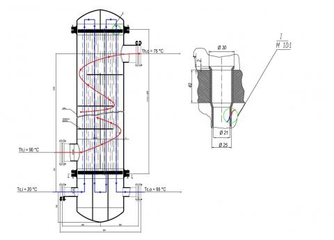
In the work [9], we calculated the corresponding shell-and-tube heat exchanger for the classical method, using the criterion equations, Nusselt numbers and a new method, using formulas (2, 3, 4, 5, 6, 7, 8). The calculation error was only 0.05 % [9]. The heat exchanger chosen and calculated by us in the work [9] has such technical characteristics (Figure 1).

Figure 1. The scheme of shell-and-tube heat exchanger (number of passes – z = 4; number of pipes – n = 206;)

The exchanger has parameters: With the heat surface area A = 97 m², D = 0.6 m, z = 4, n/z = 51.5; n = 206, L = 6 m. The area А_с = 4.5∙10^-2 m² (the cross-sectional area space between the tubes of the heat exchanger; Table 2.3 [11]). Inner diameter of pipes – d_in = 21.10^-3 m. Outside diameter of the pipes – d_out = 25.10^-3 m. Cold milk is circulated in the pipes and hot water is circulated between pipes.

Using formulas (2, 3, 4, 5, 6, 7, 8), in [9], using the formula (8), we calculated the total heat transfer coefficient of the chosen heat exchanger, having previously calculated the thermal resistances of all zones of coolants flows [9].

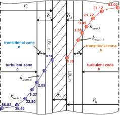
$U_δ={(\frac{r_h-δ_h}{k_{turb.h}} +\frac{δ_h}{k_{trans.h}} +\frac{δ_w}{k_w} +\frac{δ_c}{k_{trans.c}} +\frac{r_c-δ_c}{k_{turb.c}} +R_{poll})}^{-1}=$

${(\frac{124.962⋅10^{-4}}{43.02}+\frac{3.751⋅10^{-6}}{3.387}+\frac{2⋅10^{-3}}{17.5}+\frac{3.678⋅10^{-5}}{2.09}+\frac{104.632⋅10^{-4}}{58.69}+\frac{2}{3000})}^{-1}=788.7 W.m^{-2} . K^{-1}$ (8)

In the formula (8) we introduced the numerical values of the thermal resistances of all these zones (Figure 2).

Figure 2. The scheme for contacting cold milk with hot water through a metal wall with the values of turbulent thermal conductivities in heat carriers streams

Table 1. Percentage of thermal resistances of the corresponding zones of heat carriers for water and milk, respectively (Figure 2)

Parameters	Formula	Values
Thermal resistance of the turbulent zone of hot water:	$\frac{r_h-δ_h}{k_{turb.h}}$	22.9 %
Thermal resistance of the LBL zone of hot water:	$\frac{δ_h}{k_{trans.h}}$	0.087 %
Thermal resistance of the metal boundary wall:	$\frac{δ_w}{k_w}$	9.0 %
Thermal resistance of the LBL zone of cold milk:	$\frac{δ_c}{k_{trans.c}}$	1.387 %
Thermal resistance of the turbulent zone of cold milk:	$\frac{r_c-δ_c}{k_{turb.c}}$	14.06 %
Thermal resistance of contamination on both sides of the metal wall:	Rpoll	52.57 %

From this calculation it follows that the thermal resistance of the turbulent zones of cold milk and hot water is almost 37 % of the total system resistance. Add to this 52.57 % of the thermal resistance of pollution, it is almost 90 % of the thermal resistance. In addition, almost 9 % of the thermal resistance falls on the metal separation wall, and only about 1.5 % is the thermal resistance of the LBL.

Table 2. Specific thermal resistivity of the corresponding zones of heat carriers for water and milk, respectively (Figure 2) 

Parameters	Formula	Values, $\frac{m^0k}{w}$
Specific thermal resistivity of the turbulent zone of hot water	$\frac{1}{k_{turb.h}}$	23.24.10-3
Specific thermal resistivity of the LBL zone of hot water	$\frac{1}{k_{trans.h}}$	295.253.10-3
Specific thermal resistivity of the metal boundary wall	$\frac{1}{k_w}$	0.571.10-4
Specific thermal resistivity of the LBL zone of cold milk	$\frac{1}{k_{trans.c}}$	748.47.10-3
Specific thermal resistivity of the turbulent zone of cold milk	$\frac{1}{k_{turb.c}}$	17.04.10-3

As can be seen from the above analysis, the resistance of turbulent zones makes a significant contribution to the overall resistance of the shell-and-tube heat exchanger and is 23 % and 14 % for the pipes and between pipes, respectively. The specific resistance of LBLs reaches the highest values (Table 2), however, the total thermal resistance of these zones is small due to the fact that their average thickness is very small and amounts for cold milk (c): $δ_c=3.678⋅10^{-5}m$ and for hot water (h): $δ_h=3.751⋅10^{-6}m$ [9].

3.2 The dominant factors affecting the turbulent thermal conductivity of the turbulent zone of the coolant flow

Today, the most difficult problems of heat and mass transfer, in particular in the theory of plasma, are solved with the help of the method of dimensional analysis [12]. We use this method in our research.

Let us consider the functional dependence of the turbulent heat conductivity of the coolant flow on a number of factors that, in our opinion, are dominant (9):

$k_{turb.}=f(μ_{turb.},V,σ,C_P,(r-Δ),(^0K))$

$k_{turb.}=B(μ_{turb.}^X⋅V^Y⋅σ^Z⋅C_P^М⋅(r-Δ)^E(^0K)^s)$ (9)

We perform a dimensional analysis of the functional dependence (9). All the thermo-physical quantities are represented in terms of the main dimensions of quantities - mass, linear size, time and temperature [kg, m, s, ⁰K].

${{k}_{turb.}}-\left[ W.{{m}^{-1}}.{{K}^{-1}}=N.m.{{s}^{-1}}.{{m}^{-1}}.{{K}^{-1}}=kg.m.{{s}^{-3}}.{{K}^{-1}} \right]$;

${{\mu }_{turb.}}-\left[ \text{Pa}.\text{s }=N.s.{{m}^{-2}}=kg.{{m}^{-1}}.{{s}^{-1}} \right]$;

$V-\left[ {{m}^{3}}.{{s}^{-1}} \right]$;

$\sigma -\left[ N.{{m}^{-1}}=kg.m.{{s}^{-2}}.{{m}^{-1}}=kg.{{s}^{-2}} \right]$;

${{C}_{P}}-\left[ N.m.kg{{.}^{-1}}{{K}^{-1}}=kg.{{m}^{2}}{{s}^{-2}}.k{{g}^{-1}}.{{K}^{-1}}={{m}^{2}}.{{s}^{-2}}.{{K}^{-1}} \right]$;

$(r-\Delta )-\left[ m \right]$; $^{0}K-\left[ {{K}^{1}} \right]$;

We represent the exponential equation in the form of an equation of dimensions.

\({{C}_{P}}-\left[ N.m.kg{{.}^{-1}}{{K}^{-1}}=kg.{{m}^{2}}{{s}^{-2}}.k{{g}^{-1}}.{{K}^{-1}}={{m}^{2}}.{{s}^{-2}}.{{K}^{-1}} \right];\)

\((r-\Delta )-\left[ m \right]\); \(^{0}K-\left[ {{K}^{1}} \right]\)

We present such a system of equations for the exponents, taking into account the dimensional equation.

$X+Z=1; -X+3Y+2M+E=1; -X-Y-XZ-XM=-3; Z=1-X; M=0.5X+0.5; S=M-1; S=0.5X-0.5; E=0; Y=0$;

${{k}_{turb.}}=B(\mu {{_{turb}^{X}}_{.}}\cdot V\cdot {{\sigma }^{1-X}}\cdot {{C}_{P}}^{(0.5+0.5X)}\cdot {{K}^{(-0.5+0.5X)}}(r-\Delta )):\sigma .\sqrt{{{C}_{P}}/{{1}^{0}}K}$;

Grouping all the terms and unknown powers in one unknown power of X, we obtain the equation (10):

$\frac{{{k}_{turb.}}}{\sigma \cdot {{\sqrt{{{C}_{p}}\cdot {{1}^{0}}K}}_{.}}}=B{{\left( \frac{{{\mu }_{turb.}}\sqrt{{{C}_{p}}\cdot {{1}^{0}}K}}{\sigma } \right)}^{X}}$ (10)

$σ⋅\sqrt{C_p⋅1^0 K}=k_{trans.}$– transitional thermal conductivity in the transitional zone LBL (Figure 2) [9].

The formula (10) is rewritten in the form (11), taking into account the hydrophilicity of the surface of the metal wall.

\(\frac{{{k}_{turb.}}}{\sigma \cos \theta \sqrt{{{C}_{p}}\cdot {{1}^{0}}K}}=B{{\left( \frac{{{\mu }_{turb.}}\sqrt{{{C}_{p}}\cdot {{1}^{0}}K}}{\sigma \cos \theta } \right)}^{X}}\) (11)

The left-hand side of relation (11) is the ratio of turbulent and transitional heat conductivity. The right-hand side of equation (11) is a dimensionless number-an analogue of the number of Bl, derived from our work [9]. Therefore, we will call its turbulent number Bl_turb., where the turbulent viscosity appears. It will be used for calculations not in the LBL region, as the number Bl, but in the zone of free turbulence, that is, outside the LBL area. Proceeding from equation (11), we can use Eqns. (12, 13) to find the maximum turbulent heat conductivity in the central part of the heat carrier flow.

\({{k}_{turb.}}=B{{\left( \frac{{{\mu }_{turb.}}\sqrt{{{C}_{p}}\cdot {{1}^{0}}K}}{\sigma \cos \theta } \right)}^{X}}\sigma \cos \theta \sqrt{{{C}_{p}}\cdot {{1}^{0}}K}\) (12)

\(B{{l}_{turb.}}=\frac{{{k}_{turb.}}}{{{k}_{trans.}}}=\frac{{{\mu }_{turb}}}{{{\mu }_{trans}}}=B{{\left( \frac{{{\mu }_{turb.}}\sqrt{{{C}_{p}}\cdot {{1}^{0}}K}}{\sigma \cos \theta } \right)}^{X}}\) (13)

Bl_turb.number shows the degree of turbulence of the coolant in the center of the flow (in the zone of free turbulence) with respect to turbulence in the transitional layer of the LBL. The degree of turbulence of the turbulent part of the flow will depend on the magnitude of the turbulent viscosity, which in turn depends on the flow rate of the refrigerant, ie, on its flow rate, as well as on a number of other factors. In formula (12), the unknown value of the turbulent viscosity of the coolant flow remains. Therefore, a further step in our research will be to find the law of distribution of turbulent viscosity in the volume of the coolant.

3.3 The main factors affecting the turbulent viscosity in the volumes of coolants flows in the zones of free turbulences

Let us consider the functional dependence of the turbulent viscosity of the coolant flow, which enters into formulas (12) and (13) on a number of factors that, in our opinion, are dominant. Represent this equation in the form of a function (14):

\[{{\mu }_{turb.}}=f\left( V,\sigma ,{{C}_{p}},(r-\Delta ) \right)\]

\({{\mu }_{turb.}}=B\left( {{V}^{Y}}\cdot {{\sigma }^{Z}}\cdot {{C}_{p}}^{}\cdot {{(r-\Delta )}^{E}} \right)\) (14)

We shall carry out a dimensional analysis of such a functional dependence. All the thermo-physical quantities are represented in terms of the main dimensions of quantities - mass, linear size, time and temperature [kg, m, s, ⁰K]. Dimensions are similar to the above.

We represent the exponential equation in the form of an equation of dimensions.

\[\left[ kg.{{m}^{-1}}.{{s}^{-1}} \right]=B{{\left[ {{m}^{3}}.{{s}^{-1}} \right]}^{Y}}{{\left[ kg.{{s}^{-2}} \right]}^{Z}}{{\left[ {{m}^{2}}.{{s}^{-2}}.{{K}^{-1}} \right]}^{}}{{\left[ m \right]}^{E}}{{\left[ {{K}^{1}} \right]}^{S}}\]

We represent the system of equations for the exponents with allowance for the dimensional equation.

$Z=1; 3Y+2M+E=-1; -Y-2Z-2M=-1; 2M=-1-Y; E=-2Y; 0=-M+S; S=M;$

\[{{\mu }_{turb.}}=B({{V}^{Y}}\cdot {{\sigma }^{1}}\cdot {{C}_{p}}^{(-0.5-0.5Y)}{{(r-\Delta )}^{(-2Y)}}\cdot {{K}^{(-0.5-0.5Y)}}):\frac{\sigma }{\sqrt{{{C}_{p}}\cdot {{1}^{0}}K}}\]

Having grouped all terms and unknown powers to one unknown power of Y, we obtain equation (15), taking into account the hydrophilicity of the wetting surface. For convenience, the exponent of the power of Y is automatically changed to X, since we are accustomed to such a general unknown value of X.

\(\frac{{{\mu }_{turb.}}\sqrt{{{C}_{p}}\cdot {{1}^{0}}K}}{\sigma \cos \theta }=B{{\left( \frac{V}{{{(r-\Delta )}^{2}}\sqrt{{{C}_{p}}\cdot {{1}^{0}}K}} \right)}^{X}}\) (15)

$\frac{\sigma \cos \theta}{\sqrt{C_p⋅1^0 K}}=μ_(trans.)$− coefficient of transitional viscosity in the transitional zone LBL (Figure 2) (see work [9]).

It is easy to see that in the brackets on the right-hand side of equation (15) we have the ratio of the average velocity of the flow  (the ratio of the volume flow rate of the refrigerant to the cross-sectional area of the pipes) to the value, reflecting the average velocity of the thermal motion of the coolant molecules (the value $\sqrt{C_p⋅1^0 K}$). Since the total refrigerant flow extends to all pipes, in formula (15) we need to enter the value (n/z). Then this flow rate will correspond to the flow rate in one heat exchanger tube. In addition, in formula (15) it is necessary to introduce the number Pi, since it enters the cross-sectional area of one tube and is not fixed by the method of dimensional analysis. The value of the average velocity of thermal movement of the refrigerant molecules is much higher than the average linear velocity of the refrigerant. In the right side of equation (15) the numerator must be replaced by a denominator. Then the exponent of degree X gets a minus sign. Taking into account the hydrophilicity of the surface, equation (15) takes the form (16). This equation is valid for the tubular space of the heat exchanger. For a space with a shell, equation (16) takes the form (17). In equation (17), the number Pi is not introduced, but the conditional radius is calculated from the cross-sectional area of the A_c = 4.5.10^-2 m² pass, taking into account the total number of the pipes (n = 206). The value of Δ – is the step of the radius of the coolant flow in the pipes or the conditional radius in the annular space, with which we move away from the center of the coolant flow to the wall.

\(B{{l}_{{{_{turb.}}_{c}}}}=\frac{1}{B{{l}_{c}}}{{\left( \frac{\pi {{({{r}_{c}}-\Delta )}^{2}}\frac{n}{z}\sqrt{{{C}_{p.c}}\cdot {{1}^{0}}K}}{{{V}_{c}}} \right)}^{-{{X}_{c}}}}\frac{{{\mu }_{}}\sqrt{{{C}_{p.c}}\cdot {{1}^{0}}K}}{{{\sigma }_{c}}\cos \theta }\) (16)

\(B{{l}_{{{_{turb.}}_{h}}}}=\frac{1}{B{{l}_{h}}}{{\left( \frac{\pi ({{r}_{h}}-\Delta )_{{}}^{2}n\sqrt{{{C}_{p.h}}\cdot {{1}^{0}}K}}{{{V}_{h}}} \right)}^{-{{X}_{h}}}}\frac{{{\mu }_{h}}\sqrt{{{C}_{p.h}}\cdot {{1}^{0}}K}}{{{\sigma }_{h}}\cos \theta }\) (17)

The left side of Eq. (16) is the ratio of turbulent viscosity to transitional viscosity, that is, the ratio of maximal turbulent viscosity of the coolant in the middle of the stream to the minimal in the transitional zone of LBL. This relation is a dimensionless turbulent number of Bl_turb. (Formula 13).

The right-hand side is the ratio of the quantity reflecting the average rate of thermal motion of the molecules, i.e., the maximal velocity at the molecular level, to the vectors of the average linear velocities of the motion of the carriers flow – the minimal velocities.

According to our preliminary calculations based on the choice of the heat exchanger in [11], the exponent in equation (16) is Pr_turb.с = 0.733. The exponent of X in equation (17), i.e, for the annular space – Pr_turb.h = 0.573, which agrees very well and correlates with work [3, pp. 707].

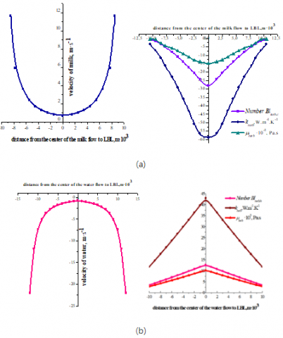
From equations (16, 17), we plotted the dependences of velocities, turbulent viscosities, thermal conductivities, as well as the turbulent numbers Bl_turb. in the tube and inter tubular space of the heat exchanger (Figure 1), i.e. showed the distributions of these thermo-physical characteristics in the volumes of the flows of heat carriers. The volumes flow rates of liquids (coolants) V_с and V_h and all other parameters included in the formulas (16, 17) we used from work [9] for the shell-and-tube heat exchanger (Figure 1) and two model liquids (milk and water). The presented graphs are undoubtedly analogues of bell-shaped curves, which obey the laws of physics surface phenomena. The graphs are the numerical values of turbulent viscosities, thermal conductivities and turbulent numbers Bl_turb. depending on the distance from the axis of the center of the pipe or the conditional center of the space between the pipes of the shell-and-tube heat exchanger (Figure 3).

Figure 3. Distribution of linear velocities $u_c$, as well as the turbulent numbers Bl_turb, turbulent viscosities $\upsilon_{turb}$ and thermal conductivities k_turb, in the volumes of the flows of model liquids-coolants: (a) – cold milk, (b) – hot water

The charts built for such parameters of the milk and water at medium temperatures of heat carriers:

\({{C}_{p.c.}}\text{= 3}.\text{914}\cdot \text{1}{{0}^{\text{3}}}\text{ J}.\text{k}{{\text{g}}^{-\text{1}}}.{{\text{K}}^{-\text{1}}}\text{ }\); \({{C}_{p.h.}}=\text{ 4}.\text{198}\cdot \text{1}{{0}^{\text{3}}}\text{ J}.\text{k}{{\text{g}}^{-\text{1}}}.{{\text{K}}^{-\text{1}}}\);

\({{\sigma }_{c}}\text{= 47}.\text{75}\cdot \text{1}{{0}^{-\text{3}}}\text{ N}.{{\text{m}}^{-\text{1}}}\); \({{\sigma }_{h}}\text{= 62}.\text{25}\cdot \text{1}{{0}^{-\text{3}}}\text{ N}.{{\text{m}}^{-\text{1}}}\);

\({{V}_{c}}\text{=}\frac{{{{\dot{m}}}_{c}}}{{{\rho }_{c}}}\text{ =11}\text{.764}\cdot \text{1}{{\text{0}}^{-3}}\text{ }{{\text{m}}^{\text{3}}}\text{.}{{\text{s}}^{\text{-1}}}\); \(Vh=\frac{{{{\dot{m}}}_{h}}}{{{\rho }_{h}}}\text{ =}34.\text{6}\cdot \text{1}{{\text{0}}^{-3}}\text{ }{{\text{m}}^{\text{3}}}\text{.}{{\text{s}}^{\text{-1}}}\);

\({{r}_{c}}\text{=10}\text{.5}\cdot \text{1}{{\text{0}}^{-3}}\text{ m  }\); \({{r}_{h}}\text{=10}\text{.0}\cdot \text{1}{{\text{0}}^{-3}}\text{ m}\);

\({{X}_{c}}\text{= }0.\text{733}\); \({{X}_{h}}=0.\text{573 }\);

\(\cos \theta =0.7-0.84\);  \(\Delta =\text{1}\text{.0}\cdot \text{1}{{\text{0}}^{-3}}\text{ m}\); \(n=206\); $z=4$;

3.4 Correlation of the proposed character of distributions of thermo-physical quantities in coolants flows with the studies of other independent authors

The nature of the distribution of thermal-physical quantities in the volume of coolants flows is similar to the experimental curves obtained by Schlichting H., Reichard H., Ludwig H., Fontmann E. et al. Which are presented in a monograph by H. Shlihting [2].

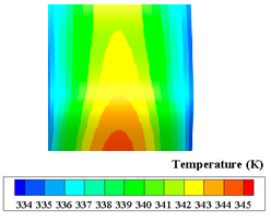
Figure 4. The distribution of the temperature field in the channel of the plate heat exchanger [13, Figure 10b]

The graphs and the nature of the changes in the turbulent viscosities, thermal conductivities, and turbulent number Bl_turb in the streams of coolants of milk and water almost completely coincide with the nature of the change in the temperature-field front, which moves in the channel of the plate heat exchanger (Figure 4). These thermo-grams were obtained in [13, Figure 10 b] by the authors Yuan Xue, Jihua Ge et al.

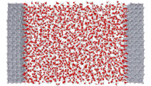
The results of our work correlate well with [14], where the authors Iype, E. et al. (2012) as a result of modeling the molecular dynamics of the water flow between two platinum plates indicate the formation of a surface monolayer, where thermal jumps and large thermal resistances arise at the boundary of platinum with water. This surface monolayer of

water molecules differ in structure from structure to volume and is associated with the action of surface forces (Figure 5).

It can be seen from the Figure 5, that the maximum specific thermal resistances occur at the boundary between silver and water. Based on our research, the maximum specific thermal resistances are also noted at the boundary of the metal wall of the heat exchanger and LBL of the heat transfer fluids (Table 2 and Figure 2).

(a)

(b)

Figure 5. Heat transfer between two platinumslabs (resembling a hannel) whih condensed layer of water: (a) Platinum slabs are atta hed with a thermostat at 300 K on the left and at 340 K on the right; (b) The distribution of temperature and density a ross the hannel. [14, Figure 4]

Formulas (12, 13 and 16, 17) completely correlate with the conclusions of the work of Maurizio Quadrio Pierre Ricco [15], where it is shown that the laminar part of the flow completely controls the turbulent part of it. The turbulent number Bl_turb,deduced by us, is responsible for the turbulent part of the flow, the multiplier $\sigma \cos \theta\sqrt{C_p⋅1^0 K}$ represents the transitional thermal conductivity in the LBL transitional zone and is responsible for the laminar and transitional part inside the LBL.

Equations (16, 17) is an undoubted analogue of equation (1), since the right part of it is the ratio of velocities, and the left is the ratio of the maximum and minimum turbulent viscosity or the maximum and minimum turbulent thermal conductivity responsible for the transfer of thermal energy, and hence the temperature in the volume of the flows of the coolants. The exponent of X is the turbulent Prandl number Pr_turb, the ratio the pulse and heat coefficients in the middle of the pipeline.

Recall that the pioneer in the study of turbulent viscosity in fluids flows is Joseph Boussinesq [16].

It should be noted that the issues of turbulent viscosity and thermal conductivity in aerodynamics of air were dealt with by Movchan V. T. et al. in the corresponding works [17, 18]. However, these questions are considered from the point of view of the mechanics of gases and liquids with the use of complex differential equations, which as Schlichting H., points out in their works, is difficult to apply for engineering calculations. Our work correlates with the above. We are considering the process of distribution of velocity and heat pulses in the case of free turbulence of liquids from the point of view of the physics of surface phenomena. The calculation of turbulent viscosities and thermal conductivities in the volume of heat carriers flows using, for example, Eqns. (12, 13, 16, 17) it seems to us rather simple.

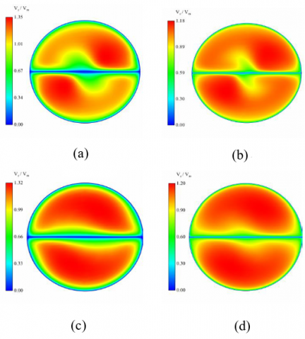
It should also be emphasized that our theoretical studies correlate well with the very vivid experiments performed in the work [19] of Parag Chaware and C.M. Sewatkar, which show the thermos-grams of the cross section of liquid flows in the pipeline at different stages of the swirler in the tube and at different Reynolds numbers (Figure 6).

The thermo-grams clearly show the LBLs near the pipe walls and near the metal surface of the swirler, whose temperature is much lower than at the center of the pipe. At higher values of Reynolds numbers, the average thickness of the LBL on thermo-grams is significantly reduced.

The positive effect of the swirler, in our opinion, is manifested in the fact that it increases the impulses of the flow rate of the refrigerant in the radial direction, allowing more intensive transfer of heat to the wall of the heat exchange surface.

Indisputable is the fact that in the volume of the liquid heat carrier there is a change in the thermal conductivity of the flow, which is distributed according to the bell-shaped law. This depends on the magnitude of the turbulent viscosity, which in turn depends on the refrigerant flow rate and the thermal-physical characteristics included in the number Bl_turb.. The change in the thermal conductivity in the volume of the turbulent fluid flow is indicated in other papers.

Our studies correlate well with the work [20], where three types of heat-conducting tubes are compared (bare, floral and hydrophilic). They are arranged in accordance with the increase in the heat transfer properties of solid surfaces and the increase in their hydrophilicity. The effect of SAS is manifested by the stronger, the more hydrophobic the surface of the tube.

In the present work, we calculated the turbulent thermal conductivities in the central parts of the coolants flows using the formulas (16 and 17). As a result, we obtained similar values of turbulent thermal conductivities, which we presented in (Figure 3) respectively blue (for milk) and red (for water) as according to calculations in our work, which we calculated from the known formulas (5, 6). This fact once again speaks of the correlation of our research with many other works of independent authors and confirms the reliability of the data obtained, contributing to the further study of the problems of heat and mass transfer in turbulent flows of liquid carriers. It should also be noted that the values of turbulent thermal conductivities in the central part of the flow of liquid heat carriers (58.82 W.m^-1.K^-1, for milk and 43.02 W.m^-1.K^-1 for water) are 2-3 times higher than the thermal conductivities, for example, stainless (17.5 W.m^-1.K^-1), and almost close to thermal conductivities, for example, carbones steels and casts irons (45 W.m^-1.K^-1). Somewhat unusual is the fact that in classical calculations of heat exchange equipment in the empirical numerical equations of Nusselt we use the values of thermal conductivities of stationary liquids, for example, for milk (0.57 W.m^-1.K^-1) and for water (0.68 W.m^-1.K^-1), which are hundreds of times less than the thermal conductivities of these liquids in areas of high turbulence. This fact suggests that the calculation of heat and mass transfer equipment according to the classical Nusselt equations is advantageous when we are dealing with well-known analogues, both equipment and heat transfer media, which transmit a quantity of heat. When, for example, nanopowders are used in coolants to improve their heat transfer properties, the application of classical methods becomes problematic. It is necessary to re-do the experiments for the appropriate coolants and heat exchangers, since the classical equations become unsuitable. In addition, such empirical equations, as a rule, are very cumbersome.

Figure 6. Axial velocity contours for the fully developed flow at (a) Y = 4 and Re = 4000 (b) Y = 4 and Re = 30000 (c) Y = 10 and Re = 4000 (d) Y = 10 and Re = 30000 [19, Figure 6]

It should also be noted that with the turbulent number Bl_turb, it is possible to select a suitable energy-efficient refrigerant in heat exchange equipment, having previously calculated the value of the turbulent viscosity in the middle of the refrigerant flow by the formulas (16, 17), or according to the well-known formula (5). In this case, we calculated the turbulence numbers Bl_turb for a number of refrigerants, which are often used in heat-exchange equipment. The results are shown in Table 3.

Values are convenient for calculation, having a known value Bl_turb (H₂0), for example, for water. Since formula (5) includes the viscosity and the Reynolds number under the root, formulas (16, 17) include turbulent viscosity and the specific heat of the refrigerant under the root in the numerator, and the surface tension coefficient in the denominator, we obtain the ratio (18):

$\frac{B{{l}_{turb(X)}}}{B{{l}_{turb({{H}_{2}}O)}}}=\frac{{{\sigma }_{({{H}_{2}}O)}}\cdot \cos {{\theta }_{({{H}_{2}}O)}}\sqrt{{{\mu }_{(X)}}\cdot {{C}_{P(X)}}}}{{{\sigma }_{(X)}}\cdot \cos {{\theta }_{(X)}}\cdot \sqrt{{{\mu }_{({{H}_{2}}O)}}\cdot {{C}_{P({{H}_{2}}O)}}}}$ (18)

Values of thermal physical values for ethylene-, propylene-, dipropylene glycols, are taken from the source [21].

An obstacle to the use of propylene- and di propylene glycols in shell-and-tube heat exchangers can be a significant decrease in Reynolds numbers due to the high dynamic viscosity coefficients. In this case, the refrigerant flow can move to the area of laminar flow regimes. Therefore, Table 3 presents the Reynolds numbers for the respective refrigerants at a given refrigerant flow rate and its flow rate, which correspond to the example of the shell-and-tube heat exchanger selected and calculated by us in the work [9]. We assume that the refrigerant moves in the space of the tubes of this heat exchanger.

Table 3. Value of the turbulent number Bl_turb (energy efficiency indicator) and Reynolds number for model liquids of water and milk and for liquid coolants at a temperature of 40 ⁰C and 5 ⁰C temperature

Liquid–phase coolant	Turbulent number Blturb. (maximal) $Bl_{turb.}=\frac{μ_{turb.}\sqrt{C_{p.}⋅1^0 K}}{σ cos\theta}$		Reynolds number $\operatorname{Re}=\frac{\upsilon d\text{ }\rho }{\mu }=\frac{\overset{.}{\mathop{4m}}\,}{\pi {{d}_{in}}n/z\cdot \mu }; $
	40 0C	5 0C	40 0C	5 0C
Water	12.48	17.96	21514	9423
Milk	21.58	29.92	12850	4383
Ethylene glycol 20 %	22.20	32.02	13857	5235
Propylene glycol 25 %	25.65	34.95	9954	2192
Dipropylene glycol 25 %	51.47	72.48	11726	2221
Propylene glycol 38 %	36.12	59.27	6254	996
Dipropylene glycol 38 %	40.40	65.16	7004	1340
Propylene glycol 47 %	42.66	73.95	5483	649
Dipropylene glycol 47 %	49.22	77.76	6327	667

As is known, the critical value of the Reynolds number for the tubular space of a shell-and-tube heat exchanger is Re_c ≈2320, and for the space between the pipes - Re_c ≈1000. Table 3 shows that most aqueous solutions of propylene- and di propylene glycols are not very suitable for use at low temperatures in shell-and-tube heat exchangers, since their values Reynolds numbers at 5 °C correspond to the laminar flow regime, where the overall heat transfer coefficients will have low values, and their use at such temperatures is inefficient. When cooling food and convenience foods, plate heat exchangers should be used, in which the corrugated plates turbulize the refrigerant flows, and the critical value of Reynolds numbers corresponds to Re_c ≈50. An exception may be shell-and-tube heat exchangers with special turbulizing inserts, the application of which was studied in the work [22]. These inserts significantly reduce the critical value of the Reynolds number, but the use of such inserts is also problematic due to the increased hydraulic resistance and difficult access to cleaning the pipes and spiral metal swirlers. The distribution of turbulent viscosities and thermal conductivities in the channels of the corrugated plates in plate heat exchangers will be the subject of our further research.