Ebenezer O. Ige![]() | Funmilayo H. Oyelami*
| Funmilayo H. Oyelami*![]() | Moses E. Etokowoh | Olaide Y. Saka-Balogun
| Moses E. Etokowoh | Olaide Y. Saka-Balogun![]()
© 2023 IIETA. This article is published by IIETA and is licensed under the CC BY 4.0 license (http://creativecommons.org/licenses/by/4.0/).
OPEN ACCESS
Rotator-cuff tear and vascular-related stenosis are common diseases in the elder persons. A balloon-like rotator-cuff is proscribed as the usual clinical intervention. Recently, computational schemes are being sought to enhance clinical outcomes in vascular-related repairs. This paper presents a numerical treatment of asymmetrically-shaped gold-embedded nanoparticle in stenotized conduit under the influence of magnetic field. We described the dynamics of fluid and particle transport under externally imposed field effect using established mathematical formulations. Thereafter, a robust numerical scheme built around spectra-relaxation scheme to implement the solution over conformation in the Au-blood stream under magnetic field imposition.
rotator-cuff, nanometer-sized fluid, spectra scheme, homotopy analysis, stenosis
Cardiovascular related disease is regarded as an issue of public health concern across the world [1]. The current hospitalization rate across the world implicates 2019-nCov as a respiratory disease which translates to cardiovascular complicity. Cardiovascular-related death is expected to surge beyond the predicted metrics by the end of year 2030 [2-4]. Thus, the coronavirus pandemic has disproportionately leading to mortality of persons with underlining cardiovascular-related diseases across race and gender in middle as well as high-income countries [5]. This contributing fact compounds the present disease burden associated to cardiovascular diseases (CVD) reported as 17.7 million deaths accounting for 31% death world-wide [6, 7]. Of all CVD deaths, atherosclerosis is associated with an estimate of 45.1% with substantial healthcare budget devoted to clinical intervention and investigation to ameliorate the severity of disease burden tied to atherosclerosis [8].
Post cardiac interventions in the coronary arteries are reported to cause a complication described as restenosis. The precise and sustain dosing of anti-proliferative materials in the region of dilated arterial vessel is considered a dependable technique to limit the severity of the balloon-like envelope injury. Recent developments in nano-medicine, biocompatible nanoparticle mediation are being deployed to engulf anti-proliferative agents which may be tailored for controlled-release of the therapeutic materials. Certain nanoparticles identified within the class of anti-proliferative agents for restenosis is documented in the report [9-11]. Notable candidate nanomaterial are classified as either lipid-based, polymer based and gel-based with respective examples as liposomal or polylactic-coglycolic acid (PLGA) nanoparticles (NPs) [12-14], poly (ethylene oxide) and poly (d.L-lactic-co-glycolic acid) [15], hydrogel spheres made of poly (N-isopropylacrylamide) [16, 17]. In addition to controlled-drug release application, NPs have been shown a promising material in prognostic intervention of atherosclerosis. For instance, image-based diagnosis of myocardial infraction employs nanoparticle because they can be embed reagents and ensure target release on the sight of disease lesion either for dosing of drugs or for providing contrast for imaging procedure. Particularly in NP-based fluorescence imaging based on fluorescence molecular tomography utilizes NPs to target macrophage specific sites in region of atherosclerosis [18]. The target deposition of therapeutic materials could be achieved using NPs in the intra-arterial region to limit the incidence of restenosis in surgical setting [10]. There are on-going computational endeavors to describe restenosis process in coronary stenosis leveraging on molecular dynamics techniques [19].
Computational techniques to handle hemodynamics of blood flow in nanoparticle-mediated systems are been reported in recent literatures. Nadeem and Ijaz [20] studied numerical investigation on nanoparticle dynamics in a venture-like orientation of arterial stenosis which showed significant pressure impedance which increased with Darcy parameter with thermal field within the diverging section of the vessel considered. Premised on these findings, the same group [21] demonstrated the dominance of metallic copper-base nanoparticle embedded in blood flow in a stenotic conduit. The impact of permeability on conjugated of nanoparticle-blood flow in a multilayered stenosis was investigated. In a latter study, Ardahaie et al. [22] presented the analysis of nanoparticle-containing blood flow under the influence of magnetic field using a combination of Akbar-Ghanji method and differential transformation method over the set of governing equations. Within the confinement of magnetic field, the authors reported that increment in Grashof parameter and negative pressure gradient precipitate the flow field while the combined effect of Brownian-thermophoretic parameters regulated the concentration and thermal behavior in the nanoparticle-blood flow field. Akbar [23] demonstrated that in a symmetrically tapered stenotic condition, the inclusion of metallic nanoparticle in water as base fluid was studied to describe flow behavior during wall shearing and resistive impedance in various sections of the region of arterial stenosis. There is convincing experimental report that NP-coated drug in the domain of vessel stenosis could be guided toward target delivery in a magnetic field environment [24-28]. Hence, the numerical study of Badfar et al. [29] described the dynamics of droplet formation and vortex generation in a magnetic field drug targeting and dispensing intervention using Fe3O4–based nanoparticle in arterial stenosis of specified geometric constrictions. Ahmed and Nadeem [30] showed that varying configuration of shaped nanoparticle of metallic copper could be modeled to describe angioplasty using mathematical techniques of perturbation approximation to estimated balloon rise of angioplasty procedure in a model catheterized stenotic blood flow. Ayub et al. [31] observed reduction in hemodynamic response considering flexible wall analogy of arterial blood vessel experiencing benign stenosis with balloon in the presence of copper-based nanoparticle-blood as conjugated fluid exhibiting viscous behavior.
The presence of stenotic complicate vascular pathways, this geometric feature impacts on the flow dynamics of plasma and its containing biomolecules constitute some grade of intricacies. Hence, a fascinating dynamics of biogenic fluid through this complex bio environment has continued to draw researchers’ attention. Reddy et al. [32] numerically considered a homogenous treatment of coupled-stress problem showing the dynamics tapered constrictions in a stenosis-plagued arterial vessel. The study highlighted the impact of stenotic configuration on pulsating flow under selected physiological conditions. In the attempt to investigate stenotic flow, Akbar et al. [33] described blood flow as a Jefferry-type non-Newtonian fluid using perturbation scheme to numerically analyze wall shear and shearing stress in the stenotic conformations of the model vascular conduit. A detailed review of numerical study and implications of the flow regime as a tool to enhancing medical procedures and improving clinical outcomes is contained in the works of Zhang et al. [34].
Some studies have shown the capability of numerical techniques to handle clinical images of stenosis diagnosis. This image-based numerical modeling has been applauded as a precursor for achieving real-time computer-driven clinical medicine. Skopalik et al. [35] presented a robust numerical assessment to predict pressure drop using image-based data in a scenario of iliac-type arterial stenosis. However, there are certain issues limiting the utilization of image-computing in a numerical scheme in the cases of arterial stenosis [36]. The ease of accessing geometric intricacies in a digital image and its contribution to boundary conditions in the formulations is slim. A deal of sensitivity is required in image-based numerical modeling to sufficient capture the geometric intricacies in a stenotic environment. To improve on sensitivity in image-based computational study, the use of nanoparticle is proposed based on the fluorescent characteristic of the some particulate metal oxides. For instance, in a bid to optimize computer tomography procedure, gold nanoparticle (AuNP) being a contrast agent was employed to improve the outcome of imaging of atherosclerosis [37]. AuNP could assist in controlling imaging procedure which could in turn improve the definition of geometrics as a precursor to defining approximation solutions at the boundary of the stenotic regions. While the boundary-defining role of particulate AuNP embedded in vascular fluids, the impact of field imposition is as well identified as tool for remote monitoring directing the swimming of the particulate solids in the fluid media [38-40]. Numerical approaches are presently being explored in nanoparticle-based fluid mechanics. For instance, Badfar et al. [41] developed a scheme based on finite volume method for magnetic drug targeting in a two-phase dynamics in a stenotic arterial vessel to predict droplet formation and vortices propagation.
This study examines a near-native scenario of the arterial vessels, we treated the stenotic conduit to a realist asymmetrical wall distension occasioned by lesion. Hence, this study explored the strength of numerical technique to describe hemodynamics of NP-mediated blood flow within modeled microenvironment of arterial restenosis. Particular emphasis on asymmetrically-constricted arterial dilation to sufficiently scrutinize transport behavior of eluting NP is made during this investigation. The study addressed three geometric conformations of AuNP in the eluting dynamics under magnetic field effect in the modeled cylindrical micro conduit.
The following are the equations which dictate mass, momentum, and energy conservation.
Δ.ˉv=0 (1)
ρηfDˉvDt=−ΔP+μηfΔ2ˉv+g(ργ)ηf(θ−θ1) (2)
ρcpDˉvDt=KΔ2θ+Qo (3)
dˉvrdr+ˉvrr1rdˉvrdr+ˉvrcosψb+rcosψbb+rcosψdˉvzdz=0 (4)
ρηf(dˉvrdr+ˉvrdˉvrdr+ˉvψrdˉvrdψ+ˉvzbb+rcosψdˉvrdz−ˉv2ψr−ˉv2zcosψb+rcosψ)=−dPdr
+μηf[(d2ˉvrdr2+1rdˉvrdr+1r2d2ˉvrdψ2)+b2(b+rcosψ)2d2ˉvrdz2−ˉvrr2dˉvrdψ+bb+rcosψ(cosψdˉvrdr+ˉvψsinψr−sinψrdˉvrdψ)−2bsinψ(b+rcosψ)2dˉvzdz−cosψ(b+rcosψ)2(ˉvrcosψ−ˉvψsinψ)]] (5)
ρηf(dˉvψdt+ˉvrdˉvψdr+ˉvψrdˉvψdψ+ˉvzbb+rcosψdˉvψdz+ˉvrˉvψr+ˉvz2cosψb+rcosψ)=−1rdPdψ+μηf
[(d2ˉvψdr2+1rdˉvψdr+1r2d2ˉvψdψ2)+b2(b+rcosψ)2d2ˉvψdz2−ˉvrr2+2r2dˉvrdψ+cosψb+rcosψdˉvψdψ−sinψ(b+rcosψ)(ˉvrr+1rdˉvψdψ)2bsinψ(b+rcosψ)2dˉvzdzsinψ(b+rcosψ)2(ˉvrcosψ−ˉvψsinψ)] (6)
ρηf(dˉvzdt+ˉvrdˉvzdr+ˉvψrdˉvzdψ+ˉvzbb+rcosψdˉvzdz−ˉvψ2r+ˉvz(ˉvrcosψ−ˉvψsinψ)b+rcosψ)
=−b(b+rcosψ)dPdzμηf[(d2ˉvzdr2+1rdˉvzdr+1r2d2ˉvzdψ2)+b2(b+rcosψ)2d2ˉvzdz2−ˉvz(b+rcosψ)2+2bb+rcosψ(cosψdˉvzdr−sinψrdˉvzdψ)+g(ργ)ηf(θ−θ1)] (7)
(ρcp)ηf(dθdt+ˉvrdθdt+ˉvzbb+rcosψdθdz)=Kηf(dθ2dr2+1rdθdr+cosψ(b+rcosψ)2d2ˉvψdz2+Qo) (8)
Introducing boundary conditions:
ˉv′′z=0 at r=h(z′′),ˉv′′z=0 at r=R(z′′,t′′)
˜θ′′=˜θ′′1 at r=h(z),˜θ′′=˜θ′′o at r=R(z′′,t′′)
The following thermo physical properties are used in this study:
μηf=1(1−Θ)2.5;μηf=Kηf(ρcp)ηf;
ρηf=(1−Θ)ρf+Θρs(ργ)ηf=(1−Θ)(ργ)f+Θ(ργ)s;
(ρcp)ηf=(1−Θ)(ργ)f+Θ(ργ)s;
KηfKf=Ks+(1+m)Kf−Θ(1+m)(Ks−Kf)Ks+(1+m)Kf+Θ(Ks−Kf) (9)
where, vr and vz which are in radial and axial directions are velocity components of the nanofluid, ef is the density, ηf is viscosity, μf is thermal expansion coefficient, (ρcp)f is the heat capacitance, Kf is the thermal conductivity of the base fluid, ρs is density, γs is thermal expansion coefficient, (ρcp)s is the heat capacitance, Ks is the thermal conductivity of materials constituting of Au-nanoparticles; ϕ is the nanofluid volume fraction, T is the temperature of the nanofluid, Q0 is the heat absorption/generation constant, B0 is the magnetic field strength, ρref is reference density, μref is the reference viscosity, Kref reference thermal conductivity and γref is the reference thermal expansion coefficient and , (ρcp)ref is the reference heat capacitance. The following non dimensional quantities are used to obtain the simplified governing equations:
[r=R∞r′′;z=L∞ˆz;ˉvr=δu∞L∞ˉv′′rˆvr;ˉvz=u∞ˉv′′z;τrz=u∞μfR∞τrz′′;ϵ=R∞b;P=P′′L∞u∞μfR∞2;Gr=ρf2gγfR∞2(θ−θo)u∞μf;β=QoR∞2Kf(θ−θo);Re=R∞u∞ρfμf;˜θ=θ−θoθi−θo;˜t=R∞t′′;˜θ=˜θ′′] (10)
Using the dimensionless terms, transformed continuity equation becomes:
δ[dˉv′′rdr′′+ˉv′′rr′′1r′′dˉv′′rdr′′+ˉv′′rcosψ1+ϵr′′cosψ]+bb+ϵr′′cosψdˉv′′zdz′′=0 (11)
ρηf(δu∞L∞R∞dˉv′′rdt′′+(δu∞)2L∞R∞ˉv′′rdˉv′′rdr′′+ϵδu∞2L∞2R∞(1+ϵr′′cosψ′′)ˉv′′zdˉv′′zdz′′−u∞2v′′2zϵcosψ′′R∞(1+ϵr′′cosψ′′))
=ρηf(δu∞L∞R∞dˉv′′rdt′′+(δu∞)2L∞R∞ˉv′′rdˉv′′rdr′′+ϵδu∞2L∞2R∞(1+ϵr′′cosψ′′)ˉv′′zdˉv′′zdz′′−u2∞v′′2zϵcosψ′′R∞(1+ϵr′′cosψ′′))
=μfL∞u∞L∞R∞3dP′′dr′′+μf(δu∞L∞R∞2d2ˉv′′rdr′′+δu∞r′′L∞R∞2dˉv′′rdr′′+1r′′2R∞2δu∞L∞d2ˉv′′rdψ′′−δu∞L∞R∞2ˉv′′rr′′+1(1+ϵr′′cosψ′′)δu∞L∞3d2ˉv′′rdZ′′2+ϵR∞(1+ϵr′′cosψ′′)[δu∞L∞R∞cosψ′′dˉv′′rdt′′−δu∞L∞R∞cosψ′′r′′dˉv′′rdr′′]+2ϵ3sinψ′′(1+ϵr′′cosψ′′)2u∞L∞dˉv′′zdz′′−ϵcosψ′′R∞2(1+ϵr′′cosψ′′)2u∞L∞ˉv′′rϵcosψ′′) (12)
Divide through by δu∞L∞R∞:
ρηfρfReϵ3(δ∧dˉv′′rdt′′+δ∧ˉvr′′dˉv′′rdr′′+δ∧ˉv′′r(1+ϵr′′cosψ′′)dˉvz′′dz′′−ϵ3ˉv′′rcosψ′′(1+ϵr′′cosψ′′))
=−dP′′dr′′+μηfμf[(δ∧ϵ2d2ˉv′′rdz′′+δ∧ϵ2r′′d2ˉv′′rdψ′′2−δ∧ϵ2ˉv′′rr′′+δ∧ϵ4(1+ϵr′′cosψ′′)d2ˉv′′zdz′′2+δ∧ϵ4(1+ϵr′′cosψ′′))(cosψ′′dˉv′′rdr′′−sinψ′′r′′dˉv′′rdψ′′+2ϵ3sinψ′′(1+ϵr′′cosψ′′)2dˉv′′zdz′′−δϵ3ˉv′′rcos2ψ′′(1+ϵr′′cosψ′′)2)] (13)
Similarly, Eq. (6) can be transformed as:
ρηfρfϵ2ˉv′′zsinψ′′1+ϵr′′cosψ′′=−1r′′dP′′dr′′+μηfμfδ∧ϵ2d2ˉv′′rdz′′2
−δ∧ϵ2ϵsinψ′′1+ϵr′′cosψ′′ˉv′′rr′′+2ϵ3sinψ′′(1+ϵr′′cosψ′′)2dˉv′′Zdz′′+δ∧ϵ4sinψ′′cosψ′′(1+ϵr′′cosψ′′)2 (14)
z-coordinate of the momentum equation become:
Reϵρηfρf(dˉv′′zdt′′+δ∧ˉv′′zdˉv′′zdr′′+ˉv′′z(1+ϵr′′cosψ′′)dˉv′′rdr′′+δ∧ˉv′′rˉv′′zcosψ′′(1+ϵr′′cosψ′′))
=−1(1+ϵr′′cosψ′′)dP′′dz′′+μηfμf(d2ˉv′′zdr′′2+1r′′dˉv′′zdr′′+1r′′d2ˉv′′zdr′′+ϵ2(1+ϵr′′cosψ′′)2d2ˉvz′′dr′′2−ϵ2ˉv′′z(1+ϵr′′cosψ′′)2+ϵcosψ′′1+ϵr′′cosψ′′dˉv′′zdr′′−ϵcosψ′′r′′(1+ϵr′′cosψ′′)dˉv′′zdψ′′+2ϵ2cosψ′′(1+ϵr′′cosψ′′)2dˉv′′rdz′′+(ργ)ηf(ργ)fGr(ψ′′)) (15)
Similarly,
RePrϵ(dθdt′′+δ∧ˉv′′rdθdr′′+sinθ(1+r′′cosψ′′)dθdz′′)=KrefKf(ρcp)f(ρcp)ref(∂2θ∂r′′+1rdθdr′′+ϵcosψ′′(1+r′′cosψ′′)dθdr′′)+ϵ2(1+r′′cosψ′′)2∂2θ∂z′′+β(ρcp)f(ρcp)ref (16)
We subject the term δ∗=δR0 representing unsteady flow of nano fluid stenosis such that R0L0≅O(1).
Also, asymmetrical stenotic conformations in the rotator-cuff balloon is represented [30] by:
R(z′′,t′′)={[R∞−2δ(cos(2πz′′−ϕ2−lo4)−7100cos(32π−ϕ−lo2))]ΩR∞Ω(t′′) for :z′′≤ϕ≥z′′+L∞ (17)
Time-varying parameter within the stenotic arena is defined as:
Ω(t′′)=1−λ(cosωt′′−1)e−λωt′′ (18)
Also:
dPdr=0
dPdψ=0
1(1+ϵrcosψ)dPdz=μηfμf(d2ˉvrdr2+1rdˉvrdr+1r2d2ˉvrdr2−m2ˉvz(1+ϵrcosψ)2+ϵcosψ1+ϵrcosψdˉvzdr−ϵsinψ1+ϵrcosψdˉvzdψ)
+(ργ)ηf(ργ)fGrψ−M2ˉvz (19)
d2θdr2=1rdθdr+ϵsinψ1+ϵrcosψdθdr+KS+2Kf+2Θ(Kf−KS)KS+2Kf−2Θ(Kf−KS)β=0 (20)
The non-dimensionless transformed system of partial differential equations is solved in this section using the spectral relaxation method (SRM). SRM is an iterative procedure that employs the Gauss–Siedel type of relaxation approach to linearize and decouple the system of coupled differential equations [42, 43]. The resulting non-linear differential equations are further discretized and solved with the Chebyshev pseudo-spectral method over the well-defined colocation points. The linear terms in each equation are evaluated at the current iteration level (denoted by r+1) and the non-linear terms are assumed to be known from the previous iteration level (denoted by r). The following are the basic steps of the method: (1) decoupling and rearrangement of the governing non-linear equations in a Gauss–Siedel manner. (2) discretizing the linear differential equations. (3) solving the discretized linear differential equations using the finite difference method.
Implementing spectra relaxation method on the latter:
L=1(1+ϵrcosψ)dPdz;a1=μηfμf;a2=μηfμf1r;
a3=μηfμf1rd(ˉvz)ndr;a4=μηfμfm2(ˉvz)n(1+ϵrcosψ)2;
a5=μηfμfϵsinψ1+ϵrcosψ;a6=(ργ)ηf(ργ)fGrψϵsinψ1+ϵrcosψ;
a7=μηfμfϵcosψ1+ϵrcosψd(ˉvz)ndr;
L=a1d2(ˉvz)n+1dr2+a2d(ˉvz)n+1dr+a3−a4+a5d(ˉvz)n+1dr+a6+a7−M2(ˉvz)n+1
d2(θ)n+1dr2=1rd(θ)n+1dr+b1d(θ)n+1dr+b2=0 (21)
Subject to: (ˉvz)n+1=0; at r=h(z); (ˉvz)n+1=0 at r=R(z,t); (θ)n+1=0; at r=h(z); (θ)n+1=0 at r=R(z,t).
The unknown functions in the resulting equation are defined using Gauss-Lobatto points defined as:
εj=cosπjN;j=0,1,2……..N;1≤ε≤−1 (22)
where, N is the number collocation points. To solve the linearized equations above, first transform the domain of the physical problem from [0, ∞]. The initial approximate for solving Eq. (20) and Eq. (21) are obtained at r=0 which are consider with preference to the boundary conditions. Hence, ˉvz0 and θ0 are chosen as:
ˉvz0=1−e−n;θ0=1−e−n (23)
Eqns. (20) and (21) are solved iteratively for the unknown functions commencing from the initial approximation (23).
The concept behind spectral collocation method is by using differentiation matrix D to approximate the derivatives of unknown variables defined:
dnˉvzdrn=∑Nk=0Dnikˉvz(εk)=Dnˉvzi=0,1,2…….Ndnθdrn=∑Nk=0Dnikθ(εk)=Dnθ,i=0,1,2…….N] (24)
a1D2(ˉvz)n+1+a2D(ˉvz)n+1+a3−a4−L+a7+a5D(ˉvz)n+1+a6−M2(ˉvz)n+1=0 (25)
D2(θ)n+1+1rD(θ)n+1+b1D(θ)n+1+b2=0 (26)
Simplifying the above:
[a1D2+a2D+a5D−M2](ˉvz)n+1+a3−a4−L+a7+a2+a6=0 (27)
[D2+1rD(θ)n+1+b1D](θ)n+1+b2=0 (28)
Now, we proceed to apply the finite difference scheme on Eqns. (27) and (28), we obtain:
[a1D2+a2D+a5D−M2](ˉvzm+1)n+1+(ˉvzm)n+12+a3−a4−L+a7+a2+a6=0
[D2+1rD+b1D](θm+1)n+1+(θm)n+12+b2=0 (29)
Simplifying further:
[a1D2+a2D+a5D−M2]2(ˉvm+1Z)n+1=−[a1D2+a2D+a5D−M2]2
(ˉvmz)n+1−a3+a4+L−a7−a2−a6 (30)
[D2+1rD+b1D]2(θm+1)n+1
=−[D2+1rD+b1D]2(θm)n+1
−b2A1(ˉvm+1z)n+1=A1(ˉvm+1z)n+1+K1B1(θm+1)n+1=B2(θm)n+1+K2] (31)
where,
A1=[a1D2+a2D+a5D−M2]2;A2=−[a1D2+a2D+a5D−M2]2B1=[D2+1rD+b1D]2;B2=−[D2+1rD+b1D]2K1=−a3+a4+L−a7−a2−a6]
The coupled partial differential equation is solved numerically, using the spectral relaxation method. Results obtained are present graphically. SRM employs the idea of Gauss-seidel relaxation approach to linearize and decoupled system of non-linear different equations. All programs are coded in MATLAB R2012a. The result was generated using the sealing parameter L=15 and we observed that increasing the value of L does not change the result to a reasonable extent.
Table 1 and 2 depict the numerical computations of velocity at a fixed point heights of stenosis for both curvature and non-curvature arteries with fixed non-dimensional parameters. It is detected that fixed value of axial velocities of brick Cu-nanoparticle, cylinder Cu-nanoparticles as well as platelet Cu-nanoparticles at heights Z=1.0, Z=1.2, for curvature K=0.1.
Table 1. Numerical computations of the velocity at critical points of the stenosis when Q∘=1.2, M=2.0, Gr=1.8, β=1.6, d=0.75, δ*=0.1 Axial velocity for M=3.9
|
R |
Z=1.0 K=0 |
Z=1.0 K=0.1 |
Z=1.2 K=0 |
Z=1.2 K=0.1 |
Z=1.71 K=0 |
Z=1.71 K=0.1 |
|
0.1 |
0.024439 |
0.018456 |
-0.051422 |
-0.061230 |
0.024439 |
0.018456 |
|
0.2 |
0.036967 |
0.028648 |
-0.006387 |
-0.006341 |
0.036967 |
0.028648 |
|
0.3 |
0.041229 |
0.034628 |
0.013492 |
0.013492 |
0.041229 |
0.0348280 |
|
0.4 |
0.043326 |
0.036472 |
0.023863 |
0.023863 |
0.043326 |
0.036472 |
|
0.5 |
0.040213 |
0.032624 |
0.027752 |
0.027752 |
0.040213 |
0.032624 |
|
0.6 |
0.036884 |
0.022146 |
0.033512 |
0.033512 |
0.036884 |
0.022146 |
|
0.7 |
0.032612 |
0.021105 |
0.025534 |
0.025534 |
0.032612 |
0.021105 |
|
0.8 |
0.021524 |
0.010122 |
0.023815 |
0.023815 |
0.021524 |
0.010122 |
|
0.9 |
0.001678 |
0.004041 |
0.015124 |
0.012703 |
0.001678 |
0.004041 |
Table 2. Numerical computations of the velocity at critical points of the stenosis when Axial velocity for M=5.0
|
R |
Z=1.0 K=0 |
Z=1.0 K=0.1 |
Z=1.2 K=0 |
Z=1.2 K=0.1 |
Z=1.71 K=0 |
Z=1.71 K=0.1 |
|
0.1 |
0.024647 |
0.018648 |
-0.051642 |
-0.061451 |
0.024647 |
0.018648 |
|
0.2 |
0.036989 |
0.028862 |
-0.006588 |
-0.006543 |
0.036989 |
0.028862 |
|
0.3 |
0.041667 |
0.034846 |
0.016224 |
0.013697 |
0.041667 |
0.034846 |
|
0.4 |
0.047214 |
0.036691 |
0.026834 |
0.023885 |
0.044214 |
0.036691 |
|
0.5 |
0.042217 |
0.032842 |
0.027971 |
0.027974 |
0.042217 |
0.032842 |
|
0.6 |
0.038686 |
0.022448 |
0.036395 |
0.033731 |
0.038686 |
0.022448 |
|
0.7 |
0.032401 |
0.021008 |
0.026771 |
0.025754 |
0.032401 |
0.021008 |
|
0.8 |
0.021322 |
0.010091 |
0.023657 |
0.023801 |
0.021322 |
0.010041 |
|
0.9 |
0.001456 |
0.004041 |
0.015042 |
0.012505 |
0.001456 |
0.004041 |
Figure 1. Variation of velocity distribution for different values of Hartman number M
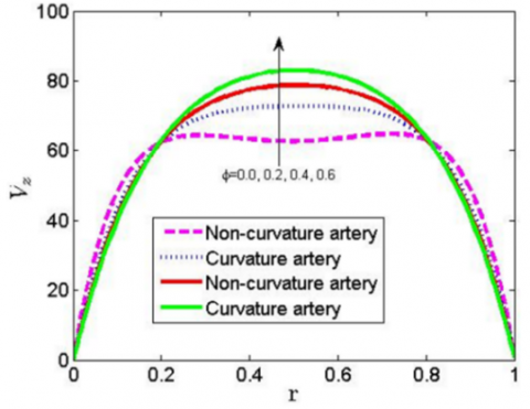
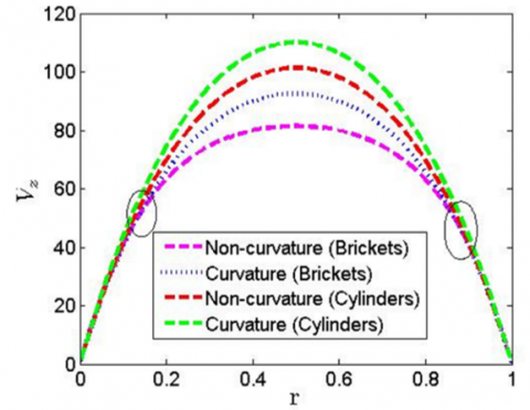
Figure 1 depicts the effort of Hartman number on the velocity distribution. It is observed that increase in the Hartman number reduces the profile. The application of the magnetic field in the opposite direction to fluid flow gives rise to a drag like force which resist the fluid velocity. Physically the magnetic field is created in the problem of fluid mechanics when an electric current is induced. The moment this current is induced probably because of the motion of an electric conducting fluid because of the presence of magnetic field in the fluid model which gives rise to this drag-like force. Figure 2 shows the effect of shape factor m of different shapes of nanoparticles (Bricks and cylinders) on the axial velocity. It is observed in the figure that axial velocity upsurges for the volume fraction parameter f=0, 0.2, 0.4, 0.1 for All-nanoparticles (M=4). It is also observed that the axial velocity close to plate and at free stream depressed. Figure 3 shows the variation of velocity profiles Vz of different values of shape factor of bricks and cylinders for all nanoparticles. The velocity of cylinder is observed to be higher than that of bricks all-nanoparticles. Arterial curvature (e=0.2) is response to the reduction of the flow but non-curvature (straight arteries) (e=0) supports the velocities of the fluid flow for different type of all-nanoparticles.
Figure 2. Variation of velocity profiles Vz for different values of all-nanoparticle volume fraction with shape factor of brinks and cylinder when shape factor (m=4)
Figure 3. Variation of velocity profiles Vz for different values of shape factor of bricks and cylinders
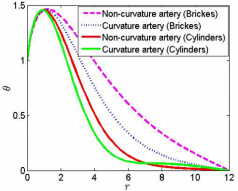
Figure 4. Variation of temperature profile with r for different values of shape factor of bricks and cylinder
Figure 4 shows the temperature profile q with r for distribution quantities of shape factor of bricks All-nanoparticles and cylinder maximum temperature than cylinder All-nanoparticles. We observed that the Bricks are having it curvature (e=0) is responsible for enhancing the temperature of nanofluid in the artery than a non-curvature artery (e=0). And non-curvature K=0 arteries respectively. It is obviously that the very close to the catheter, the axial velocity is observed to be higher for curvature artery compared to the non-curvature artery.
In this study, temperature in case of All-nanoparticles decreases close to the plate and away from the plate with comparison to the hybrid nanofluid; the nanoparticles temperature is greater than that of all-nanoparticles. Hence, the temperature decreases in the presence of hybrid nanofluid in the flows. It is worth, mentioning that the temperature is higher for trapezoidal stenosis but the bell-shaped stenosis possess lower temperature along among all other types of stenosis.
This study examined the effect of fluid flow in stenosed blood vessels with the presence of both nano particles/nano fluids and a magnetic field, and we wanted to find out if:
(1) We are able to clear blockages in blood vessels or micro conduits with the given scenario.
(2) Take note of the behaviour of the working fluid under said working scenario.
The study results have shown the following:
(1) The magnetic field moves opposite to the direction of the flow of the working fluid.
(2) Different nanoparticles have different velocity profiles. This is also due to their shape factor.
(3) Behaviour of nanoparticles is also dependent on the type of stenoses encountered.
(4) Hybrid nanoparticles have a smaller temperature profile compared to other nanoparticles.
Under the influence of magnetic fields with increasing values of r and ϕ, the velocity vz, of flow eventually becomes zero.
The authors are grateful to management of Afe Babalola University Ado-Ekiti Nigeria for providing facilities to conduct this research. The contribution of Dr. Bidemi Falodun is appreciated during the stage of this research.
|
vr |
radial directions velocity components of the nanofluid (m/s) |
|
vz |
axial directions are velocity components of the nanofluid (m/s) |
|
ef |
density (kg/ms2) |
|
ηf |
viscosity (Nsm2) |
|
μf |
thermal expansion coefficient (µmm-1K-1) |
|
(ρcp)f |
heat capacitance (mK-1) |
|
Kf |
thermal conductivity of the base fluid (Wm-1K-1) |
|
ρs |
density (kg/ms2) |
|
γs |
thermal expansion coefficient (µmm-1K-1) |
|
(ρcp)s |
heat capacitance |
|
Ks |
thermal conductivity of materials constituting of Au-nanoparticles (Wm-1K-1) |
|
ϕ |
nanofluid volume fraction (unitless) |
|
T |
temperature of the nanofluid (K) |
|
Q0 |
heat absorption/generation constant (kJ) |
|
B0 |
magnetic field strength (Am-1) |
|
ρref |
reference density (kg/ms2) |
|
μref |
reference viscosity (Nsm2) |
|
Kref |
reference thermal conductivity (Wm-1K-1) |
|
γref |
reference thermal expansion coefficient (µmm-1K-1) |
|
(ρcp)ref |
reference heat capacitance (mK-1) |
|
δ* |
unsteady flow of nanofluid stenosis (m/s) |
|
g |
gravitational acceleration, m.s-2 |
|
k |
thermal conductivity, W.m-1. K-1 |
|
Cp |
specific heat, J. kg-1. K-1 |
|
Subscripts |
|
|
p |
nanoparticle |
|
f |
fluid (pure water) |
|
nf |
Nanofluid |
|
Greek Symbols |
|
|
α |
thermal diffusivity, m2. s-1 |
|
β |
thermal expansion coefficient, K-1 |
|
ϕ |
solid volume fraction (unitless) |
|
Ɵ |
dimensionless temperature (unitless) |
|
µ |
dynamic viscosity, kg. m-1.s-1 |
|
δ |
stenosis parameter (m) |
|
µ |
viscosity (Nsm2) |
|
ϕ |
nanofluid volume fraction (unitless) |
|
Ɵ |
temperature (K) |
|
Ω |
time-varying parameter (s) |
|
∈ |
Curvature of nanoparticle (m) |
|
ρ |
Density of nanofluid (kg/ms2) |
|
λ |
Resistive impedance (unitless) |
|
τ |
shear stress (N/m) |
|
σ |
shape factor of nanoparticle (unitless) |
|
ω |
pulsating parameter of the stenoized vessel (unitless) |
|
ψ |
Angular orientation of the cylindrical-spherical (Degree) |
[1] Aje, T.O., Miller, M. (2009). Cardiovascular disease: A global problem extending into the developing world. World Journal of Cardiology, 1(1): 3. https://doi.org/10.4330/wjc.v1.i1.3
[2] Bansal, M. (2020). Cardiovascular disease and COVID-19. Diabetes & Metabolic Syndrome: Clinical Research & Reviews, 14(3): 247-250. https://doi.org/10.1016/j.dsx.2020.03.013
[3] Heidenreich, P.A., Trogdon, J.G., Khavjou, O.A., Butler, J., Dracup, K., Ezekowitz, M.D., Woo, Y.J. (2011). Forecasting the future of cardiovascular disease in the United States: A policy statement from the American Heart Association. Circulation, 123(8): 933-944. https://doi.org/10.1161/CIR.0b013e31820a55f5
[4] Paramasivam, A., Priyadharsini, J.V., Raghunandhakumar, S., Elumalai, P. (2020). A novel COVID-19 and its effects on cardiovascular disease. Hypertension Research, 43(7): 729-730. https://doi.org/10.1038/s41440-020-0461-x
[5] Clerkin, K.J., Fried, J.A., Raikhelkar, J., et al. (2020). COVID-19 and cardiovascular disease. Circulation, 141(20): 1648-1655. https://doi.org/10.1161/CIRCULATIONAHA.120.046941
[6] World Health Organization. (2017). World Health Organization (WHO)/Fact sheet/Cardiovascular diseases (CVDs). WHO.
[7] Bejarano, J., Navarro-Marquez, M., Morales-Zavala, F., Morales, J.O., Garcia-Carvajal, I., Araya-Fuentes, E., Kogan, M.J. (2018). Nanoparticles for diagnosis and therapy of atherosclerosis and myocardial infarction: evolution toward prospective theranostic approaches. Theranostics, 8(17): 4710-4732. https://doi.org/10.7150/thno.26284
[8] Cormode, D.P., Roessl, E., Thran, A., et al. (2010). Atherosclerotic plaque composition: Analysis with multicolor CT and targeted gold nanoparticles. Radiology, 256(3): 774-782. https://doi.org/10.1148/radiol.10092473
[9] McDowell, G., Slevin, M., Krupinski, J. (2011). Nanotechnology for the treatment of coronary in stent restenosis: A clinical perspective. Vascular Cell, 3(1): 1-5. https://doi.org/10.1186/2045-824X-3-8
[10] Labhasetwar, V., Song, C., Levy, R.J. (1997). Nanoparticle drug delivery system for restenosis. Advanced Drug Delivery Reviews, 24(1): 63-85. https://doi.org/10.1016/S0169-409X(96)00483-8
[11] Uwatoku, T., Shimokawa, H., Abe, K., et al. (2003). Application of nanoparticle technology for the prevention of restenosis after balloon injury in rats. Circulation Research, 92(7): e62-e69. https://doi.org/10.1161/01.res.0000069021.56380.e2
[12] Ghitman, J., Biru, E.I., Stan, R., Iovu, H. (2020). Review of hybrid PLGA nanoparticles: Future of smart drug delivery and theranostics medicine. Materials & Design, 193: 108805. https://doi.org/10.1016/j.matdes.2020.108805
[13] Chan, J.M., Rhee, J.W., Drum, C.L., Bronson, R.T., Golomb, G., Langer, R., Farokhzad, O.C. (2011). In vivo prevention of arterial restenosis with paclitaxel-encapsulated targeted lipid–polymeric nanoparticles. Proceedings of the National Academy of Sciences, 108(48): 19347-19352. https://doi.org/10.1073/pnas.1115945108
[14] Ambesh, P., Campia, U., Obiagwu, C., Bansal, R., Shetty, V., Hollander, G., Shani, J. (2017). Nanomedicine in coronary artery disease. Indian Heart Journal, 69(2): 244-251. https://doi.org/10.1016/j.ihj.2017.02.007
[15] Essa, D., Kondiah, P.P., Choonara, Y.E., Pillay, V. (2020). The design of poly (lactide-co-glycolide) nanocarriers for medical applications. Frontiers in Bioengineering and Biotechnology, 8: 48. https://doi.org/10.3389/fbioe.2020.00048
[16] Doorty, K.B., Golubeva, T.A., Gorelov, A.V., et al. (2003). Poly (N-isopropylacrylamide) co-polymer films as potential vehicles for delivery of an antimitotic agent to vascular smooth muscle cells. Cardiovascular Pathology, 12(2): 105-110. https://doi.org/10.1016/S1054-8807(02)00165-5
[17] Wessely, R. (2010). New drug-eluting stent concepts. Nature Reviews Cardiology, 7(4): 194-203. https://doi.org/10.1038/nrcardio.2010.14
[18] Kratz, J.D., Chaddha, A., Bhattacharjee, S., Goonewardena, S.N. (2016). Atherosclerosis and nanotechnology: diagnostic and therapeutic applications. Cardiovascular Drugs and Therapy, 30(1): 33-39. https://doi.org/10.1007/s10557-016-6649-2
[19] Yin, R.X., Yang, D.Z., Wu, J.Z. (2014). Nanoparticle drug-and gene-eluting stents for the prevention and treatment of coronary restenosis. Theranostics, 4(2), 175-200. https://doi.org/10.7150/thno.7210
[20] Nadeem, S., Ijaz, S. (2015). Theoretical analysis of metallic nanoparticles on blood flow through stenosed artery with permeable walls. Physics Letters A, 379(6): 542-554. https://doi.org/10.1016/j.physleta.2014.12.013
[21] Ijaz, S., Nadeem, S. (2016). Examination of nanoparticles as a drug carrier on blood flow through catheterized composite stenosed artery with permeable walls. Computer Methods and Programs in Biomedicine, 133: 83-94. https://doi.org/10.1016/j.cmpb.2016.05.004
[22] Ardahaie, S.S., Amiri, A.J., Amouei, A., Hosseinzadeh, K., Ganji, D.D. (2018). Investigating the effect of adding nanoparticles to the blood flow in presence of magnetic field in a porous blood arterial. Informatics in Medicine Unlocked, 10: 71-81. https://doi.org/10.1016/j.imu.2017.10.007
[23] Akbar, N.S. (2016). Metallic nanoparticles analysis for the blood flow in tapered stenosed arteries: Application in nanomedicines. International Journal of Biomathematics, 9(01): 1650002. https://doi.org/10.1142/S1793524516500029
[24] McBain, S.C., Yiu, H.H., Dobson, J. (2008). Magnetic nanoparticles for gene and drug delivery. International Journal of Nanomedicine, 3(2): 169. https://doi.org/10.2147/ijn.s1608
[25] Sensenig, R., Sapir, Y., MacDonald, C., Cohen, S., Polyak, B. (2012). Magnetic nanoparticle-based approaches to locally target therapy and enhance tissue regeneration in vivo. Nanomedicine, 7(9): 1425-1442. https://doi.org/10.2217/nnm.12.109
[26] Manshadi, M.K., Saadat, M., Mohammadi, M., Shamsi, M., Dejam, M., Kamali, R., Sanati-Nezhad, A. (2018). Delivery of magnetic micro/nanoparticles and magnetic-based drug/cargo into arterial flow for targeted therapy. Drug Delivery, 25(1): 1963-1973. https://doi.org/10.1080/10717544.2018.1497106
[27] Gleich, B., Hellwig, N., Bridell, H., et al. (2007). Design and evaluation of magnetic fields for nanoparticle drug targeting in cancer. IEEE Transactions on Nanotechnology, 6(2): 164-170. https://doi.org/10.1109/TNANO.2007.891829
[28] Thomsen, L.B., Thomsen, M.S., Moos, T. (2015). Targeted drug delivery to the brain using magnetic nanoparticles. Therapeutic Delivery, 6(10): 1145-1155. https://doi.org/10.4155/tde.15.56
[29] Badfar, H., Yekani Motlagh, S., Sharifi, A. (2020). Numerical simulation of magnetic drug targeting to the stenosis vessel using Fe3O4 magnetic nanoparticles under the effect of magnetic field of wire. Cardiovascular Engineering and Technology, 11(2): 162-175. https://doi.org/10.1007/s13239-019-00446-x
[30] Ahmed, A., Nadeem, S. (2017). Shape effect of Cu-nanoparticles in unsteady flow through curved artery with catheterized stenosis. Results in Physics, 7: 677-689. https://doi.org/10.1016/j.rinp.2017.01.015
[31] Ayub, M., Shahzadi, I., Nadeem, S. (2019). A ballon model analysis with Cu-blood medicated nanoparticles as drug agent through overlapped curved stenotic artery having compliant walls. Microsystem Technologies, 25(8): 2949-2962. https://doi.org/10.1007/s00542-018-4263-x
[32] Reddy, J.R., Srikanth, D., Murthy, S.K. (2014). Mathematical modelling of pulsatile flow of blood through catheterized unsymmetric stenosed artery—Effects of tapering angle and slip velocity. European Journal of Mechanics-B/Fluids, 48: 236-244. https://doi.org/10.1016/J.EUROMECHFLU.2014.07.001
[33] Akbar, N.S., Nadeem, S., Ali, M. (2011). Jeffrey fluid model for blood flow through a tapered artery with a stenosis. Journal of Mechanics in Medicine and Biology, 11(03): 529-545. https://doi.org/10.1142/S0219519411003879
[34] Zhang, J.M., Zhong, L., Luo, T., et al. (2014). Numerical simulation and clinical implications of stenosis in coronary blood flow. BioMed Research International, 2014. https://doi.org/10.1155/2014/514729
[35] Skopalik, S., Hall Barrientos, P., Matthews, J., Radjenovic, A., Mark, P., Roditi, G., Paul, M.C. (2021). Image-based computational fluid dynamics for estimating pressure drop and fractional flow reserve across iliac artery stenosis: A comparison with in-vivo measurements. International Journal for Numerical Methods in Biomedical Engineering, 37(12): e3437. https://doi.org/10.1002/CNM.3437
[36] Sturdy, J., Kjernlie, J.K., Nydal, H.M., Eck, V.G., Hellevik, L.R. (2019). Uncertainty quantification of computational coronary stenosis assessment and model based mitigation of image resolution limitations. Journal of Computational Science, 31: 137-150. https://doi.org/10.1016/J.JOCS.2019.01.004
[37] Chhour, P., Kim, J., Benardo, B., et al. (2017). Effect of gold nanoparticle size and coating on labeling monocytes for CT tracking. Bioconjugate Chemistry, 28(1): 260-269. https://doi.org/10.1021/ACS.BIOCONJCHEM.6B00566
[38] Reeves, D.B., Weaver, J.B. (2014). Approaches for modeling magnetic nanoparticle dynamics. Critical Reviews™ in Biomedical Engineering, 42(1): 85. https://doi.org/10.1615/CritRevBiomedEng.2014010845
[39] Kush, P., Kumar, P., Singh, R., Kaushik, A. (2021). Aspects of high-performance and bio-acceptable magnetic nanoparticles for biomedical application. Asian Journal of Pharmaceutical Sciences, 16(6): 704-737. https://doi.org/10.1016/J.AJPS.2021.05.005
[40] Jat, S.K., Gandhi, H.A., Bhattacharya, J., Sharma, M.K. (2021). Magnetic nanoparticles: an emerging nano-based tool to fight against viral infections. Materials Advances, 2(14): 4479-4496. https://doi.org/10.1039/D1MA00240F
[41] Badfar, H., Yekani Motlagh, S., Sharifi, A. (2020). Numerical simulation of magnetic drug targeting to the stenosis vessel using Fe3O4 magnetic nanoparticles under the effect of magnetic field of wire. Cardiovascular Engineering and Technology, 11(2): 162-175. https://doi.org/10.1007/S13239-019-00446-X
[42] Ige, E.O., Oyelami, F.H., Olutayo-Irheren, J., Okunlola, J.T. (2022). Magneto-hemodynamic of blood flow having impact of radiative flux due to infrared magnetic hyperthermia: Spectral relaxation approach. International Journal of Design & Nature and Ecodynamics, 17(5): 773-779. https://doi.org/10.18280/ijdne.170516
[43] Oyelami, F.H., Ige, E.O., Falodun, B.O., Saka-Balogun, O.Y., Adeyemo, O.A. (2022). Magneto-hemodynamics fluid hyperthermia in a tumor with blood perfusion. Mathematical Modelling of Engineering Problems, 9(5): 1210-1216. https://doi.org/10.18280/mmep.090507