Rania Khallout![]() | Maroua Grid
| Maroua Grid![]() | Salem Tegani
| Salem Tegani![]() | Adel Chala*
| Adel Chala*![]()
© 2025 The authors. This article is published by IIETA and is licensed under the CC BY 4.0 license (http://creativecommons.org/licenses/by/4.0/).
OPEN ACCESS
In this work, we introduce a hybrid method that combines Long Short-Term Memory (LSTM) neural networks with Taylor Series Expansion (TSE) to solve high-dimensional Fredholm Integral Equations of the second kind (SFIEs). Specifically, we focus on systems with up to 10000 dimensions, which are common in fields like fluid dynamics, electromagnetics, and quantum mechanics. Traditional methods for solving these equations, such as discretization, collocation, and iterative solvers, face significant challenges in high-dimensional spaces due to their computational cost and slow convergence. LSTM networks approximate the solution functions, and Taylor Series Expansion refines the approximation, ensuring higher accuracy and computational efficiency. Numerical experiments demonstrate that the hybrid method significantly outperforms traditional approaches in both accuracy and stability. This method provides a promising approach to solving complex high-dimensional integral equations efficiently in scientific and engineering applications.
computational complexity, convergence rate, Fredholm Integral Equations, high-dimensional systems, hybrid method, Long Short-Term Memory (LSTM), numerical solutions, Taylor Series Expansion (TSE)
Fredholm Integral Equations (FIEs) of the second kind are fundamental in a wide range of scientific disciplines, including fluid dynamics, electromagnetics, and quantum mechanics, where they describe systems involving unknown functions embedded within integrals. These equations are essential for modeling various physical phenomena, such as heat conduction, electromagnetic wave propagation, and wave scattering [1]. However, solving FIEs, particularly in high-dimensional spaces, presents significant computational challenges due to the nonlinear nature of these equations. As the number of variables increases, obtaining accurate solutions becomes increasingly difficult with traditional numerical methods [2].
Traditional approaches for solving high-dimensional FIEs, such as discretization techniques (finite difference, finite element methods), collocation methods, and iterative solvers—encounter significant limitations as the problem dimensionality increases [3]. Discretization methods, although effective in lower-dimensional spaces, require a large number of grid points to approximate the solution, resulting in computationally expensive, large-scale matrices [4]. Collocation methods, which approximate the solution by evaluating integrals at specific points, suffer from exponential growth in the number of evaluation points as the number of dimensions increases [5]. Iterative approaches, such as the Nyström method, tend to converge slowly in high-dimensional spaces, requiring many iterations and prolonged computational time [6]. These limitations underscore the need for more efficient techniques capable of addressing the complexities of large-scale FIEs.
Recent advancements in machine learning, particularly the use of Long Short-Term Memory (LSTM) networks, have shown promising potential for solving high-dimensional integral equations. LSTMs, a specialized form of recurrent neural networks (RNNs), are adept at capturing complex, nonlinear relationships in high-dimensional data, making them suitable candidates for solving Fredholm Integral Equations [7]. However, despite their ability to handle high-dimensional functions, LSTMs often struggle with precision, particularly in scientific applications where high accuracy is required [8]. This challenge necessitates the development of new methodologies that combine the strengths of machine learning and traditional numerical techniques.
To overcome the limitations of LSTM networks, we propose a hybrid method that combines the power of LSTM networks with the precision of Taylor Series Expansion (TSE). The Taylor Series Expansion provides a reliable initial approximation of the solution, which is then iteratively refined by the LSTM network, improving both the accuracy and computational efficiency of the solution [9]. This hybrid approach leverages the advantages of both techniques: LSTMs can handle high-dimensional data, while the Taylor series enhances the precision of the solution, leading to faster convergence and more accurate results. Preliminary experiments indicate that this hybrid approach significantly outperforms traditional methods in terms of accuracy and computational performance [10].
In addition to LSTM-based methods, Taylor Series Expansion (TSE) has been explored for solving FIEs. Huabsomboon et al. [11] explored Taylor-series expansion methods specifically for second-kind FIEs, showing their potential in solving these types of equations efficiently. Furthermore, Jiang and Xu [12] applied deep learning to solve oscillatory FIEs, presenting a deep learning-based approach for such problems. Zappala et al. [13] extended this by leveraging neural integral equations to learn integral operators, improving the capability of neural networks in solving complex integral equations. Moghaddam et al. [14] introduced an advanced physics-informed neural network with residuals, improving the accuracy of solutions for complex integral equations. Additionally, Lu et al. [15] proposed a neural network algorithm using sine-cosine basis functions and extreme learning machines for approximating solutions to various classes of Fredholm and Volterra integral equations. Kumar and Ravi Kanth [16] explored the use of tension splines in the computational study of time-dependent singularly perturbed parabolic partial differential equations, which share similarities with FIEs in terms of their complexity and solution methods. Saha Ray and Sahu [17] proposed numerical methods for solving second-kind Fredholm integral equations, contributing significantly to the body of work on these equations. Sabzevari [18] reviewed several numerical solution techniques for nonlinear Volterra-Fredholm integral equations, highlighting hybrid methods to improve solution accuracy and efficiency. Lastly, Afiatdoust et al. [19] introduced a hybrid-based numerical method for solving systems of mixed Volterra-Fredholm integral equations, offering a new approach to solving complex integral equations. Micula and Milovanović [20] also provided an in-depth study on iterative processes and integral equations of the second kind, highlighting the mathematical foundations and methods for solving these types of equations efficiently.
This paper introduces the hybrid LSTM-Taylor Series Expansion approach for solving high-dimensional FIEs. The structure of the paper is as follows: Section 2 provides an overview of traditional methods for solving FIEs. Section 3 details the proposed hybrid method, including its mathematical foundations and implementation. Section 4 presents numerical experiments comparing the performance of the hybrid method with traditional approaches. Finally, Section 5 concludes the paper, discussing the advantages, limitations, and potential future directions of this hybrid approach.
2.1 Problem formulation
Consider the system of Fredholm Integral Equations of the second kind:
$f_i(x)=g_i(x)+\lambda \sum_{j=1}^n \int_a^b K_{i j}(x, y) f_j(y) d y, \quad i=1,2, \ldots, n$
where, fi(x) are the unknown functions, gi(x) are known functions, Kij(x, y) is the kernel function, λ is a constant (scaling factor), and $x, y \in[a, b]$ are the variables.
The goal is to find the functions fi(x) that satisfy the above system of equations.
2.2 Taylor Series Expansion (TSE) approach
Taylor Series Expansion approach for solving a linear system of Fredholm integral equations of the second kind as a numerical method. This method reduces the system of integral equations to a linear system of ordinary differential equations. After including boundary conditions, this system reduces to a system of equations that can be solved easily by any usual methods. That study is an extension of the work presented in paper [21].
Consider the LSFIE2 defined by:
$\begin{aligned} & \left(\begin{array}{l}y_1(x) \\ y_2(x) \\ \vdots \\ y_n(x)\end{array}\right)=\left(\begin{array}{l}f_1(x) \\ f_2(x) \\ \vdots \\ f_n(x)\end{array}\right) \\ & +\lambda \int_0^1\left(\begin{array}{llll}k_{1,1}(x, t) & k_{1,2}(x, t) & \cdots & k_{1, n}(x, t) \\ k_{2,1}(x, t) & k_{2,2}(x, t) & \cdots & k_{2, n}(x, t) \\ \vdots & \vdots & & \vdots \\ k_{n, 1}(x, t) & k_{n, 2}(x, t) & \cdots & k_{n, n}(x, t)\end{array}\right)\left(\begin{array}{l}y_1(t) \\ y_2(t) \\ \vdots \\ y_n(t)\end{array}\right)\end{aligned}$
Or
$y_i(x)=f_i(x)+\lambda \sum_{j=1}^n \int_0^1 k_{i, j}(x, t) y_j(t) d t$ (1)
where, i=1, 2, …, n and 0≤x≤1.
A Taylor Series Expansion can be made for the solution of yj(t) in Eq. (1):
$\begin{gathered}y_j(t)=y_j(x)+y_j^{\prime}(x)(t-x)+\cdots+\frac{1}{m!} y_j^{(m)}(t- x)^m+E(t)\end{gathered}$ (2)
where, E(t) is the error between yj(t) and its Taylor Series Expansion in Eq. (2), we use the first m term of Eq. (2):
$\begin{gathered}y_i(x)=f_i(x)+\lambda \sum_{j=1}^n \int_0^1 k_{i, j}(x, t) \sum_{r=0}^m \frac{1}{r!}(t- x)^r y_j^{(r)}(x) d t+\lambda \int_0^1 \sum_{j=1}^n k_{i, j}(x, t) E(t) d t\end{gathered}$ (3)
We neglect the term containing E(t) that is $\lambda \int_0^1 \sum_{j=1}^n k_{i, j}(x, t) E(t) d t$, then substituting Eq. (2) into Eq. (1), we get:
$\begin{aligned} &\left(\begin{array}{l}y_1(x) \\ y_2(x) \\ \vdots \\ y_n(x)\end{array}\right) \simeq\left(\begin{array}{l}f_1(x) \\ f_2(x) \\ \vdots \\ f_n(x)\end{array}\right) +\lambda \sum_{r=0}^m \frac{1}{r!} \int_0^1(t-x)^r\left(\begin{array}{lll}k_{1,1}(x, t) & \cdots & k_{1, n}(x, t) \\ k_{2,1}(x, t) & \cdots & k_{2, n}(x, t) \\ \vdots & & \vdots \\ k_{n, 1}(x, t) & \cdots & k_{n, n}(x, t)\end{array}\right)\left(\begin{array}{l}y_1^{(r)}(x) \\ y_2^{(r)}(x) \\ \vdots \\ y_n^{(r)}(x)\end{array}\right) d t\end{aligned}$ (4)
$\begin{gathered}y_i(x) \simeq f_i(x) +\lambda \sum_{j=1}^n \sum_{r=0}^m \frac{1}{r!} y_j^{(r)}(x) \int_0^1 k_{i, j}(x, t)(t-x)^r d t\end{gathered}$ (5)
then,
$\begin{gathered}y_i(x) -\lambda \sum_{j=1}^n \sum_{r=0}^m \frac{1}{r!} y_j^{(r)}(x)\left[\int_0^1 k_{i, j}(x, t)(t-x)^r d t\right] \simeq f_i(x)\end{gathered}$ (6)
Eq. (6) becomes a linear system of (ODE) ordinary differential equations that we have to solve. For solving the linear system of (ODE) in Eq. (6), we need an appropriate number of boundary conditions. In order to construct boundary conditions, we first differentiate s terms both sides of Eq. (1) with respect to x, that is:
$\begin{gathered}y_i^{(s)}(x)=f_i^{(s)}(x)+\lambda \sum_{j=1}^n \int_0^1 k_{i, j}^{(s)}(x, t) y_j^{(s)}(x) d t \\ i=1,2, \ldots, n\end{gathered}$ (7)
where, $k_{i, j}^{(s)}(x, t)=\frac{\partial k_{i, j}^{(s)}(x, t)}{\partial x^{(s)}}, s=1,2, \ldots, m$.
Applying the mean value theorem for integral in Eq. (7), yields:
$f_i^{(s)}(x) \simeq y_i^{(s)}(x)-\lambda\left[\sum_{j=1}^n \int_0^1 k_{i, j}(x, t) d t\right] y_j(x)$ (8)
Now, the combination of Eq. (6) and Eq. (8) leads to: AY=F.
The previous system (AY=F), is a linear system of algebraic equations (for more details see Appendix), this system can be solved analytically or numerically.
2.2.1 Numerical example for solving LSFIE’2 using TSE
Consider the following linear system of Fredholm integral equations of the second kind with the exact solutions (y1(x), y2(x)) = (x, x2).
$\left\{\begin{array}{l}y_1(x)=\frac{11}{6} x-\frac{11}{15}-\int_0^1(x+t) y_1(t) d t-\int_0^1\left(x+2 t^2\right) y_2(t) d t \\ y_2(x)=\frac{5}{4} x^2+\frac{1}{4} x-\int_0^1 x t^2 y_1(t) d t-\int_0^1 x^2 t y_2(t) d t\end{array}\right.$,
Applying TSE to previous system, we get the following system:
$$\left(\begin{array}{llll}x+\frac{3}{2} & \frac{1}{3}-x^2 & x+\frac{2}{3} & x+\frac{2}{3} \\1 & \frac{3}{2}-x & 1 & 1 \\\frac{x}{3} & \frac{x}{4}-\frac{x^2}{3} & 1+\frac{x^2}{2} & 1+\frac{x^2}{2} \\\frac{1}{3} & \frac{1}{4}-\frac{x}{3} & x & x\end{array}\right)\left(\begin{array}{l}y_i(x) \\y_i^{\prime}(x) \\\vdots \\y_i^{(s)}(x)\end{array}\right)=\left(\begin{array}{l}\frac{11}{6} x+\frac{11}{15} \\\frac{11}{6} \\\frac{5}{4} x^2+\frac{1}{4} x \\\frac{5}{2} x+\frac{1}{4}\end{array}\right)$$
A Y=F
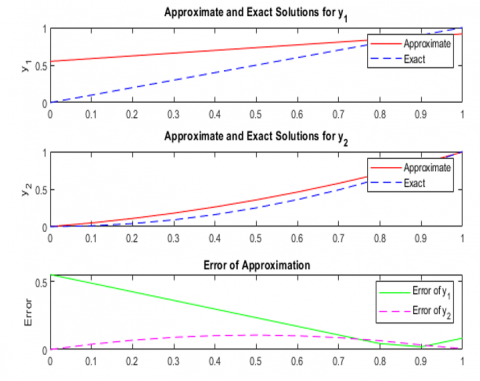
This ordinary differential equations are solved approximately using the Gauss algorithm. A comparison of the approximate and exact solutions for y1(x) and y2(x), derived from Taylor Series Expansion (TSE), is shown in Table 1 and Figure 1 illustrates the approximation versus the exact solution for SFIE’2 using TSE.
In traditional methods such as Taylor Series Expansion (TSE) for solving Fredholm Integral Equations of the second kind (FIE2), various limitations become evident, especially when dealing with high-dimensional or complex systems. These limitations are primarily related to issues such as computational complexity, slow convergence, and instability, which can hinder the effectiveness of TSE in these contexts. A detailed overview of these challenges is provided in Table 2, which summarizes the key drawbacks associated with traditional TSE approach.
Figure 1. Approximation solutions vs exact solution of LSFIE’2 using TSE
Table 1. Approximate solutions of y1(x) and y2(x) vs exact solutions using TSE
|
x |
Solution y1(x) |
Solution y2(x) |
||||
|
|
Exact |
Approximate |
Errorapp |
Exact |
Approximate |
Errorapp |
|
0 |
0.0000 |
0.5500 |
0.5500 |
0.0000 |
0.0000 |
0.0000 |
|
0.1 |
0.1000 |
0.5867 |
0.4867 |
0.0100 |
0.0486 |
0.0386 |
|
0.2 |
0.2000 |
0.6233 |
0.4233 |
0.0400 |
0.1085 |
0.0685 |
|
0.3 |
0.3000 |
0.6600 |
0.3600 |
0.0900 |
0.1796 |
0.0896 |
|
0.4 |
0.4000 |
0.6967 |
0.2967 |
0.1600 |
0.2621 |
0.1021 |
|
0.5 |
0.5000 |
0.7333 |
0.2333 |
0.2500 |
0.3558 |
0.1058 |
|
0.6 |
0.6000 |
0.7700 |
0.1700 |
0.3600 |
0.4608 |
0.1008 |
|
0.7 |
0.7000 |
0.8067 |
0.1067 |
0.4900 |
0.5771 |
0.0871 |
|
0.8 |
0.8000 |
0.8433 |
0.0433 |
0.6400 |
0.7047 |
0.0647 |
|
0.9 |
0.9000 |
0.8800 |
0.0200 |
0.8100 |
0.8436 |
0.0336 |
|
1 |
1.0000 |
0.9167 |
0.0833 |
1.0000 |
0.9937 |
0.0063 |
Table 2. Limitations of traditional methods (TSE) for solving a system of Fredholm integral equations of the second kind (FIE’2)
|
Limitation |
Description |
Example in Numerical Solution |
|
Computational Complexity |
As the number of unknown functions increases, the system becomes larger, resulting in higher computational costs. |
The inclusion of higher-order Taylor series terms significantly increases the computational burden, as seen in the growing size of the system in the numerical example. |
|
Accuracy-Efficiency Trade-off |
Increasing the number of Taylor series terms improves the accuracy but also raises the computational effort. |
The error reduces with more terms, but the required computational time also grows, as illustrated by the increasing error for larger x in the numerical results. |
|
Error Propagation |
Higher-order Taylor expansions introduce error accumulation, which can reduce the reliability of the solution. |
The error increases as higher-order terms are added, particularly visible in the growing discrepancy between exact and approximate solutions for both $y_1(x)$ and $y_2(x)$. |
|
Limited for Nonlinear Systems |
TSE is less effective for nonlinear Fredholm Integral Equations, which often require more specialized techniques. |
Nonlinear kernels or functions in the Fredholm equation would necessitate more complex methods, which TSE may not handle efficiently. |
|
Inefficiency in Large-Scale Problems |
TSE becomes inefficient as the system size and complexity increase, especially in high-dimensional problems. |
As the number of unknown functions increases in the numerical example, TSE becomes computationally impractical for large-scale problems. |
3.1 Formulate the problem
High-dimensional system of Fredholm Integral Equations of the second kind is given by:
$f_i\left(x_j\right)=g_i\left(x_j\right)+\lambda \sum_{k=1}^N \int_a^b K_{i j}\left(x_j, y_k\right) f_j\left(y_k\right) d y, \quad i=1,2, \ldots, n$
here, gi(xj): Known function; Kij(xj, yk): Known kernel; fj(yk): Unknown function to be solved.
3.2 Discretization
The integral equation is first discretized using numerical quadrature methods (e.g., Gaussian quadrature):
$f_i(\mathbf{x}) \approx g_i(\mathbf{x})+\lambda \sum_j K_i\left(\mathbf{x}, \mathbf{y}_j\right) \cdot \mathbf{u}\left(\mathbf{y}_j\right) \Delta y_j$.
where,
3.3 Training data
To train the LSTM network, synthetic training data is generated by sampling the points x and y from the domain. The process is as follows:
• Known Analytical Functions: We select known analytical test cases for fi(x), such as polynomials, exponentials, or trigonometric functions. These known functions are chosen because their exact forms allow comparison with the LSTM model outputs.
• Integral Equation Evaluation: For each of these test functions, we solve the Fredholm integral equation using numerical methods (such as Gaussian quadrature) to evaluate the integrals. The resulting fi(xj) values form the training data.
• Discretization: We discretize the domain [a, b] into a set of points, solving the equation over these points and pairing the resulting fi(xj) values with their corresponding input points x and y.
• Noise and Perturbations: To simulate real-world scenarios, random noise is added to the training data to prevent over-fitting and improve the generalization capability of the model.
• LSTM Training: The generated pairs (x, fi(x)) are used to train the LSTM model, which learns the mapping between x and fi(x).
3.4 LSTM network architecture
The LSTM model is designed to approximate u(y):
• Input Layer: Accepts a vectorized form of x, y, and Ki(x, y). Each input feature is normalized to ensure consistent scaling for effective learning.
• Embedding Layer: For higher-dimensional input data, an optional embedding layer can reduce dimensionality while preserving essential information.
• Recurrent Layers: Multiple LSTM layers are stacked to model the complex dependencies in the integral equation.
• Dropout Regularization: Dropout layers prevent overfitting by randomly deactivating a fraction of neurons during training.
• Fully Connected Layers: A dense neural network maps the output of the recurrent layers to the target u(y).
• Output Layer: Outputs the predicted u(y), which can be a scalar or vector.
• Activation Functions: ReLU or tanh are used for nonlinearity; linear activation is applied in the output layer.
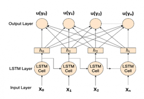
The architecture of the LSTM model is illustrated in Figure 2, which provides a detailed visualization of the network's structure.
Figure 2. LSTM model architecture
3.5 Loss function
The loss function is defined based on the residual of the integral equation:
Loss $=\sum_i\left\|f_i(\mathbf{x})-g_i(\mathbf{x})-\lambda \sum_j K_i\left(\mathbf{x}, \mathbf{y}_j\right) \cdot u\left(\mathbf{y}_j\right) \Delta y_j\right\|^2$.
3.6 Testing and validation
Evaluate the trained LSTM on test data and compare its predictions for u(y) against analytical or numerical solutions.
|
Algorithm 1: Solving High-Dimensional SFIEs ‘2 using LSTM. |
|
Initialize Parameters: Set the number of iterations N. Define g0(x)=g(x). n=0 to N-1 Step 1: Compute an approximation: $\tilde{f}_n(x)=g_n(x)+\lambda \int_D K(x, z) \tilde{f}_n(z) d z$ Step 2: Train the LSTM to solve the FIE and approximate fn(x): $f_n(x)=\operatorname{LSTM}\left(x ; \mathbf{W}, \mathbf{B}_n\right)$ Step 3: Update gn+1(x) for the next iteration: $g_{n+1}(x)=g(x)+\lambda \int_D K(x, z)\left(g\left(f_n(z)\right)-f_n(z)\right) d z$ Step 4: Increment n: n←n+1 Output: The final approximation f(x) for the Fredholm Integral Equation. |
4.1 Formulate the problem
High-dimensional Fredholm Integral Equations of the second kind are given by:
$\begin{gathered}f_i\left(x_j\right)=g_i\left(x_j\right)+\lambda \sum_{k=1}^N \int_a^b K_{i j}\left(x_j, y_k\right) f_j\left(y_k\right) d y, \\ i=1,2, \ldots, n\end{gathered}$
where, fi(xj) are the unknown functions we need to solve for; gi(xj) are known functions; Kij(xj, yk) are the kernel functions; λ is a constant.
4.2 Taylor Series Expansion approximation
In order to approximate the solution of the Fredholm Integral Equation using a hybrid LSTM and Taylor Series Expansion, we utilize a Taylor Series Expansion around a known point, say x0, for the unknown functions fj:
$f_j\left(y_k\right) \approx f_j\left(x_0\right)+\frac{d f_j}{d x}\left(x_0\right)\left(y_k-x_0\right)+\frac{1}{2} \frac{d^2 f_j}{d x^2}\left(x_0\right)\left(y_k-x_0\right)^2+\cdots$
This approach enables us to approximate the integrals more effectively and reduce computational complexity.
4.3 Discretization
The integral in the Fredholm equation is discretized using a numerical quadrature method such as Gaussian quadrature. However, we also incorporate Taylor Series Expansions for each term in the integral to achieve more accurate solutions. The discretized equation becomes:
$f_i(\mathbf{x}) \approx g_i(\mathbf{x})+\lambda \sum_j K_i\left(\mathbf{x}, \mathbf{y}_j\right)\left[f_j\left(x_0\right)+\frac{d f_j}{d x}\left(x_0\right)\left(y_j-x_0\right)+\cdots\right] \Delta y_j$
4.4 Training data
The synthetic training data for the Hybrid LSTM-TSE approach is generated by:
• Known Analytical Functions: Similar to the LSTM approach, we use known analytical test functions for fi(x), such as polynomials, exponentials to generate synthetic data.
• Integral Equation Evaluation: For each test function, the Fredholm integral equation is solved numerically by applying quadrature methods and generating data points.
• Taylor Series Expansion: As in the LSTM approach, Taylor Series Expansions are used to generate an initial approximation of the unknown functions. These approximations help improve the LSTM’s performance.
• Discretization: The domain is discretized, and the equation is solved over these points to generate input-output pairs for the LSTM model.
• Noise and Perturbations: Noise is introduced into the training data to simulate real-world uncertainties and improve the robustness of the model.
• LSTM Training: The LSTM model is trained on these synthetic data pairs (x, fi(x)) and incorporates Taylor series terms to iteratively refine the solution.
4.5 Hybrid LSTM-TSE model
The model is trained as follows:
$f_j\left(y_k\right) \approx \operatorname{LSTM}\left(y_k ; \mathbf{W}, \mathbf{B}_j\right)+$ TaylorSeriesExpansionTerms $\left(y_k\right)$
where, the LSTM model predicts the unknown function fj(yk), and the Taylor Series Expansion accounts for the variations in the values of fj at different points.
4.6 Loss function
The loss function is defined as the residual error between the actual solution and the predicted solution, incorporating the Taylor series approximation. For each equation i, we minimize:
Loss $=\sum_i \| f_i(\mathbf{x})-g_i(\mathbf{x})-\lambda \sum_j K_i\left(\mathbf{x}, \mathbf{y}_j\right)\left[u\left(\mathbf{y}_j\right)+\right.$ TaylorExpansionTerms $] \Delta y_j \|^2$
4.7 Testing and validation
Evaluate the trained Hybrid on test data and compare its predictions for u(y) against analytical or numerical solutions.
|
Algorithm 2: Solving High-Dimensional SFIEs'2 using LSTM-TSE. |
|
Initialize Parameters: Set the number of iterations N. Define initial guess f0(x)=g(x) for the unknown function. Define the Taylor Series Expansion terms for each fj(yk): $\begin{gathered}f_j\left(y_k\right) \approx f_j\left(x_0\right)+\frac{d f_j}{d x}\left(x_0\right)\left(y_k-x_0\right)+\frac{1}{2} \frac{d^2 f_j}{d x^2}\left(x_0\right)\left(y_k\right. \left.-x_0\right)^2+\cdots\end{gathered}$ Define the known kernel Kij(xj, yk) and function gi(xj). Define the regularization parameter λ. n=0 to N'-1 Step 1: Compute an approximation of fn(x): $\tilde{f}_n(x)=g_n(x)+\lambda \sum_j K\left(x, y_j\right) \tilde{f}_n\left(y_j\right) \Delta y_j$ Apply Taylor expansion to approximate the unknown function fn(yj) at each point yj: $\begin{aligned} & f_n\left(y_j\right) \approx \operatorname{LSTM}\left(y_j ; \mathbf{W}, \mathbf{B}_n\right)+\text { TaylorSeriesExpansionTerms }\end{aligned}$ Step 2: Update the known function g(n+1)(x): $\begin{gathered}g_{n+1}(x)=g(x)+\lambda \sum_j K\left(x, y_j\right)\left[\operatorname{LSTM}\left(f_n\left(y_j\right)\right)-\right. \left.f_n\left(y_j\right)\right] \Delta y_j\end{gathered}$ Step 3: Train the LSTM model to approximate fn(x) using the residual error: $\begin{gathered}\operatorname{Loss}_n=\sum_i \| f_i(\mathbf{x})-g_i(\mathbf{x})-\lambda \sum_j K_i\left(\mathbf{x}, \mathbf{y}_j\right)\left[u\left(\mathbf{y}_j\right)+\right.\text { TaylorExpansionTerms }] \Delta y_j \|^2\end{gathered}$ Step 4: Update LSTM weights W, Bn using gradient descent based on the computed loss: $\mathbf{W}, \mathbf{B}_n \leftarrow \mathbf{W}-\alpha \nabla_{\mathbf{W}}{Loss_{n}}, \quad \mathbf{B}_n \leftarrow \mathbf{B}_n-\alpha \nabla_{\mathbf{B}_n} \operatorname{Loss}_n$ Step 5: Increment n for the next iteration: n←n+1 Output: The final approximation f(x) for the Fredholm Integral Equation. |
In this section, we present the outcomes obtained from applying the LSTM approach and the Hybrid LSTM-TSE approach to solve High-dimensional SFIEs’2 and analyze their performance in comparison to each other.
5.1 LSTM approach
The LSTM approach involves training a Long Short-Term Memory (LSTM) model to predict the unknown function u(y) given the kernel function K(x, y) and known functions fi(x). The model learns the relationship between these inputs through a training process, and once trained, the LSTM approximates the solution of the High-Dimensional SFIEs’2.
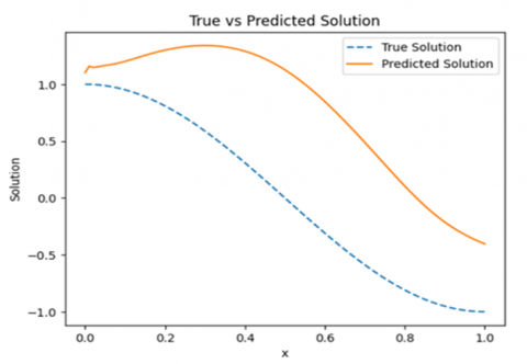
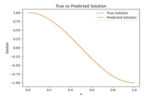
Figure 3. The solutions of high-dimensional SFIEs’2 using LSTM
After training the LSTM-TSE model (Algorithm 1), we first compare its predictions with the analytical or numerical reference solution. The plot of the true solution alongside the predicted solution in Figure 3 is a key indicator of how well the model generalizes to unseen data.
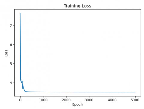
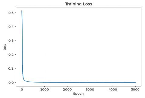
The loss function curve, shown in Figure 4, is a crucial indicator of the model's training process and its ability to minimize errors. The curve shows the decrease in error as the model iterates over the training data.
Figure 4. The loss function computed by Algorithm 1
5.2 Hybrid LSTM-TSE approach
In the Hybrid LSTM-Taylor Series Expansion Approach, an initial guess for the unknown function u(y) is provided by a Taylor Series Expansion. This initial guess is then refined by the LSTM model, which uses the kernel K(x, y) and known functions fi(x) to iteratively improve the solution.
Figure 5. The solutions of high-dimensional SFIEs’2 using hybrid LSTM-TSE approach
After training the Hybrid LSTM-TSE approach (Algorithm 2), we compare its predictions with the known analytical or numerical solutions to assess its accuracy, as shown in Figure 5. The following observations were made:
The behavior of the loss function during training is an important indicator of the model’s learning process and its ability to reduce errors, as shown in Figure 6.
Figure 6. The loss function computed by the Hybrid LSTM-TSE approach
5.3 Comparison criteria
The table above (Table 3) summarizes the key differences between the two approaches. The Hybrid LSTM-Taylor Series Expansion Approach generally provides better accuracy, faster convergence, and greater efficiency, especially for high-dimensional problems. This is because the Taylor Series Expansion gives more detailed information of starting points for the LSTM, reducing the need for large amounts of training data and computational resources. On the other hand, the LSTM approach is more reliant on the quality and quantity of training data and may face challenges in high-dimensional spaces due to the curse of dimensionality.
Table 3. Comparison of the LSTM approach with hybrid LSTM-TSE approach
|
Criteria |
LSTM Approach |
Hybrid LSTM-TSE Approach |
|
Accuracy |
High, but depends on data quality and training time |
Generally higher due to better initial guess |
|
Computational Efficiency |
Computationally expensive, especially in high dimensions |
Faster convergence due to Taylor series starting point |
|
Convergence Rate |
Slower, especially for complex or high-dimensional problems |
Faster convergence due to informed initial guess |
|
Applicability to High-Dimensional Problems |
Struggles due to curse of dimensionality |
More efficient due to the Taylor expansion providing a good starting guess |
|
Interpretability |
Low, as LSTM is a black-box model |
Higher, due to the analytical Taylor expansion |
The Hybrid LSTM-Taylor Series Expansion (TSE) Approach represents a significant advancement in solving high-dimensional Fredholm Integral Equations (FIEs). By combining the adaptive learning capabilities of Long Short-Term Memory (LSTM) networks with the precision of Taylor Series Expansion, the method enhances both convergence speed and accuracy, addressing the computational challenges posed by traditional numerical techniques. This synergy between machine learning and analytical methods offers an efficient solution for complex integral equations, ensuring both computational feasibility and mathematical rigor.
However, despite its advantages, the approach has inherent limitations. Computational cost remains a key concern, particularly during the training phase of the LSTM model. The resources required for training, such as memory and processing power, increase significantly for high-dimensional problems, which may hinder the scalability of the method in some cases. Additionally, while the method is more efficient than traditional solvers in handling high-dimensional problems, it still faces dimensional constraints. As the dimensionality of the problem increases, the number of training data points required grows exponentially, which can lead to longer training times and higher computational demands. Furthermore, the effectiveness of the model is dependent on the availability of reliable synthetic training data, which may not always be feasible for all problem domains.
In conclusion, the Hybrid LSTM-TSE Approach is a powerful and promising tool for solving Fredholm Integral Equations more accurately and efficiently. While computational and dimensional challenges remain, the approach provides a strong framework for tackling high-dimensional problems, with continued advances in machine learning and computational power likely to further enhance its applicability.
Solving SFIEs’2 Using Taylor Series Expansion (TSE) Approach
Taylor Series Expansion approach for solving a linear system of Fredholm integral equations of the second kind as a numerical method. This method reduces the system of integral equations to a linear system of ordinary differential equations. After including boundary conditions, this system reduces to a system of equations that can be solved easily by any usual methods. That study is an extension of the work presented in paper [21].
Consider the LSFIE2 defined by:
$\begin{aligned} & \left(\begin{array}{l}y_1(x) \\ y_2(x) \\ \vdots \\ y_n(x)\end{array}\right)=\left(\begin{array}{l}f_1(x) \\ f_2(x) \\ \vdots \\ f_n(x)\end{array}\right) +\lambda \int_0^1\left(\begin{array}{llll}k_{1,1}(x, t) & k_{1,2}(x, t) & \cdots & k_{1, n}(x, t) \\ k_{2,1}(x, t) & k_{2,2}(x, t) & \cdots & k_{2, n}(x, t) \\ \vdots & \vdots & & \vdots \\ k_{n, 1}(x, t) & k_{n, 2}(x, t) & \cdots & k_{n, n}(x, t)\end{array}\right)\left(\begin{array}{l}y_1(t) \\ y_2(t) \\ \vdots \\ y_n(t)\end{array}\right)\end{aligned}$
$y_i(x)=f_i(x)+\lambda \sum_{j=1}^n \int_0^1 k_{i, j}(x, t) y_j(t) d t$ (A1)
where, i=1, 2, …, n and 0≤x≤1.
A Taylor Series Expansion can be made for the solution of yj(t) in Eq. (A1):
$\begin{gathered}y_j(t)=y_j(x)+y_j^{\prime}(x)(t-x)+\cdots+\frac{1}{m!} y_j^{(m)}(t- x)^m+E(t)\end{gathered}$ (A2)
where, E(t) is the error between yj(t) and its Taylor Series Expansion in Eq. (A2), we use the first m term of Eq. (A2):
$\begin{aligned} & \left(\begin{array}{l}y_1(x) \\ y_2(x) \\ \vdots \\ y_n(x)\end{array}\right)=\left(\begin{array}{l}f_1(x) \\ f_2(x) \\ \vdots \\ f_n(x)\end{array}\right) +\lambda \int_0^1\left(\begin{array}{lll}k_{1,1}(x, t) & \cdots & k_{1, n}(x, t) \\ k_{2,1}(x, t) & \cdots & k_{2, n}(x, t) \\ \vdots & & \vdots \\ k_{n, 1}(x, t) & \cdots & k_{n, n}(x, t)\end{array}\right)\left(\begin{array}{l}y_1(x)+\cdots+\frac{1}{m!} y_1^{(m)}(t-x)^m+E(t) \\ y_2(x)+\cdots+\frac{1}{m!} y_2^{(m)}(t-x)^m+E(t) \\ \vdots \\ y_n(x)+\cdots+\frac{1}{m!} y_n^{(m)}(t-x)^m+E(t)\end{array}\right) d t\end{aligned}$
$\begin{gathered}y_i(x)=f_i(x)+\lambda \sum_{j=1}^n \int_0^1 k_{i, j}(x, t) \sum_{r=0}^m \frac{1}{r!}(t- x)^r y_j^{(r)}(x) d t+\lambda \int_0^1 \sum_{j=1}^n k_{i, j}(x, t) E(t) d t\end{gathered}$ (A3)
We neglect the term containing E(t) that is $\lambda \int_0^1 \sum_{j=1}^n k_{i, j}(x, t) E(t) d t$, then substituting Eq. (A2) into Eq. (A1), we get:
$\begin{aligned} & \left(\begin{array}{l}y_1(x) \\ y_2(x) \\ \vdots \\ y_n(x)\end{array}\right) \simeq\left(\begin{array}{l}f_1(x) \\ f_2(x) \\ \vdots \\ f_n(x)\end{array}\right) +\lambda \int_0^1\left(\begin{array}{lll}k_{1,1}(x, t) & \cdots & k_{1, n}(x, t) \\ k_{2,1}(x, t) & \cdots & k_{2, n}(x, t) \\ \vdots & & \vdots \\ k_{n, 1}(x, t) & \cdots & k_{n, n}(x, t)\end{array}\right)\left(\begin{array}{l}\sum_{r=0}^m \frac{1}{r!}(t-x)^r y_1^{(r)}(x) \\ \sum_{r=0}^m \frac{1}{r!}(t-x)^r y_2^{(r)}(x) \\ \vdots \\ \sum_{r=0}^m \frac{1}{r!}(t-x)^r y_n^{(r)}(x)\end{array}\right)\end{aligned}$
$\begin{gathered}\left(\begin{array}{l}y_1(x) \\ y_2(x) \\ \vdots \\ y_n(x)\end{array}\right) \simeq\left(\begin{array}{l}f_1(x) \\ f_2(x) \\ \vdots \\ f_n(x)\end{array}\right) +\lambda \sum_{r=0}^m \frac{1}{r!} \int_0^1(t-x)^r\left(\begin{array}{lll}k_{1,1}(x, t) & \cdots & k_{1, n}(x, t) \\ k_{2,1}(x, t) & \cdots & k_{2, n}(x, t) \\ \vdots & & \vdots \\ k_{n, 1}(x, t) & \cdots & k_{n, n}(x, t)\end{array}\right)\left(\begin{array}{l}y_1^{(r)}(x) \\ y_2^{(r)}(x) \\ \vdots \\ y_n^{(r)}(x)\end{array}\right) d t\end{gathered}$ (A4)
$y_i(x) \simeq f_i(x)+\lambda \sum_{j=1}^n \int_0^1 k_{i, j}(x, t) \sum_{r=0}^m \frac{1}{r!}(t-x)^r y_j^{(r)}(x) d t$
$\begin{gathered}y_i(x) \simeq f_i(x)+ \lambda \sum_{j=1}^n \sum_{r=0}^m \frac{1}{r!} y_j^{(r)}(x) \int_0^1 k_{i, j}(x, t)(t-x)^r d t\end{gathered}$ (A5)
$\begin{gathered}y_i(x)-\lambda \sum_{j=1}^n \sum_{r=0}^m \frac{1}{r!} y_j^{(r)}(x)\left[\int_0^1 k_{i, j}(x, t)(t-\right. \left.x)^r d t\right] \simeq f_i(x)\end{gathered}$ (A6)
Eq. (A6) becomes a linear system of (ODE) ordinary differential equations that we have to solve. For solving the linear system of (ODE) Eq. (6), we need an appropriate number of boundary conditions. In order to construct boundary conditions, we first differentiate s terms both sides of (1) with respect to x, that is:
$\begin{gathered}y_i^{(s)}(x)=f_i^{(s)}(x)+\lambda \sum_{j=1}^n \int_0^1 k_{i, j}^{(s)}(x, t) y_j^{(s)}(x) d t \\ i=1,2, \ldots, n\end{gathered}$ (A7)
where, $k_{i, j}^{(s)}(x, t)=\frac{\partial k_{i, j}^{(s)}(x, t)}{\partial x^{(s)}}, s=1,2, \ldots, m$.
Applying the mean value theorem for integral in Eq. (A7), yields:
$f_i^{(s)}(x) \simeq y_i^{(s)}(x)-\lambda\left[\sum_{j=1}^n \int_0^1 k_{i, j}(x, t) d t\right] y_j(x)$ (A8)
Now Eq. (A6) combined with Eq. (A8) becomes: AY=F.
where,
$\begin{gathered}A= \left(\begin{array}{llll}1-\lambda \int_0^1 k_{i, 1}(x, t) d t & -\lambda \int_0^1 k_{i, 2}(x, t)(t-x) d t & \cdots & -\lambda \frac{1}{m!} \int_0^1 k_{i, n}(x, t)(t-x)^m d t \\ -\lambda \int_0^1 k_{i, 1}^{\prime}(x, t) d t & 1-\lambda \int_0^1 k_{i, 2}^{\prime}(x, t)(t-x) d t & \cdots & -\lambda \frac{1}{m!} \int_0^1 k_{i, n}^{\prime}(x, t)(t-x)^m d t \\ \vdots & \vdots & & \vdots \\ -\lambda \int_0^1 k_{i, 1}^{(s)}(x, t) d t & -\lambda \int_0^1 k_{i, 2}^{(s)}(x, t)(t-x) d t & \cdots & 1-\lambda \frac{1}{m!} \int_0^1 k_{i, n}^{(s)}(x, t)(t-x)^m d t\end{array}\right)\end{gathered}$
$Y=\left(\begin{array}{l}y_i(x) \\ y_i^{\prime}(x) \\ \vdots \\ y_i^{(s)}(x)\end{array}\right), \quad F=\left(\begin{array}{l}f_i(x) \\ f_i^{\prime}(x) \\ \vdots \\ f_i^{(s)}(x)\end{array}\right)$.
The previous system (AY=F), is a linear system of algebraic equations that can be solved analytically or numerically.
[1] Kress, R. (1999). Linear Integral Equations (2nd ed.). Springer. https://doi.org/10.1007/978-1-4612-0559-3
[2] Hochreiter, S., Schmidhuber, J. (1997). Long short-term memory. Neural Computation, 9(8): 1735-1780. https://doi.org/10.1162/neco.1997.9.8.1735
[3] Sun, H., Lu, Y. (2024). Numerical solutions to one-dimensional linear Volterra–Fredholm integral equations based on LS-SVM model. Journal of Computational and Applied Mathematics, 451: 116013. https://doi.org/10.1016/j.cam.2024.116013
[4] Tair, B., Slimani, W. (2024). Solving higher-order nonlinear Volterra integro-differential equations using two discretization methods. Journal of Applied Mathematics and Computing, 70: 2785-2807. https://doi.org/10.1007/s12190-024-02075-7
[5] Yang, L., Osher, S.J. (2024). PDE generalization of in-context operator networks: A study on 1D scalar nonlinear conservation laws. Journal of Computational Physics, 519: 113379. https://doi.org/10.1016/j.jcp.2024.113379
[6] Muthuswamy, V.V., Dilip, D. (2024). Advanced machine learning techniques for efficient numerical solutions of nonlinear partial differential equations in high-dimensional spaces. Mathematics for Application, 13(1).
[7] Amirfakhrian, M., Mirzaei, S.M. (2022). A modified Taylor-series for solving a Fredholm integral equation of the second kind. Mathematical Analysis and its Contemporary Applications, 4(4): 39-48. https://doi.org/10.30495/maca.2022.1956497.1056
[8] Zhang, D., Yang, L., Karniadakis, G.E. (2018). Bi-directional coupling between a PDE-domain and an adjacent data-domain equipped with multi-fidelity sensors. Journal of Computational Physics, 374: 121-134. https://doi.org/10.1016/j.jcp.2018.07.039
[9] Guan, Y., Fang, T., Zhang, D., Jin, C. (2022). Solving Fredholm integral equations using deep learning. International Journal of Applied and Computational Mathematics, 8(2): 87. https://doi.org/10.1007/s40819-022-01288-3
[10] Bassi, H., Zhu, Y., Liang, S., Yin, J., Reeves, C.C., Vlček, V., Yang, C. (2024). Learning nonlinear integral operators via recurrent neural networks and its application in solving integro-differential equations. Machine Learning with Applications, 15: 100524. https://doi.org/10.1016/j.mlwa.2023.100524
[11] Huabsomboon, P., Novaprateep, B., Kaneko, H. (2010). On Taylor-series expansion methods for the second kind integral equations. Journal of Computational and Applied Mathematics, 234(5): 1466-1472. https://doi.org/10.1016/j.cam.2010.02.023
[12] Jiang, J., Xu, Y. (2024). Deep neural network solutions for oscillatory Fredholm integral equations. Journal of Integral Equations and Applications, 36(1): 23-55. https://doi.org/10.1216/jie.2024.36.23
[13] Zappala, E., Fonseca, A.H.D.O., Caro, J.O., Moberly, A.H., Higley, M.J., Cardin, J., Dijk, D.V. (2024). Learning integral operators via neural integral equations. Nature Machine Intelligence, 6(9): 1046-1062. https://doi.org/10.1038/s42256-024-00886-8
[14] Moghaddam, M.M., Parand, K., Kheradpisheh, S.R. (2025). Advanced physics-informed neural network with residuals for solving complex integral equations. arXiv preprint. https://doi.org/10.48550/arXiv.2501.16370
[15] Lu, Y., Zhang, S., Weng, F., Sun, H. (2023). Approximate solutions to several classes of Volterra and Fredholm integral equations using the neural network algorithm based on the sine-cosine basis function and extreme learning machine. Frontiers in Computational Neuroscience, 17: 1120516. https://doi.org/10.3389/fncom.2023.1120516
[16] Kumar, P.M.M., Ravi Kanth, A.S.V. (2020). Computational study for a class of time-dependent singularly perturbed parabolic partial differential equation through tension spline. Computational and Applied Mathematics, 39: 233. https://doi.org/10.1007/s40314-020-01278-5
[17] Saha Ray, S., Sahu, P.K. (2013). Numerical methods for solving Fredholm integral equations of second kind. Abstract and Applied Analysis, 2013: 426916. https://doi.org/10.1155/2013/426916
[18] Sabzevari, M. (2019). A review on “Numerical solution of nonlinear Volterra-Fredholm integral equations using hybrid of …” [Alexandria Eng. J. 52 (2013) 551–555]. Alexandria Engineering Journal, 58(3): 1099-1102. https://doi.org/10.1016/j.aej.2019.09.012
[19] Afiatdoust, F., Hosseini, M.M., Heydari, M.H., Mohseni Moghadam, M. (2024). A hybrid-based numerical method for a class of systems of mixed Volterra–Fredholm integral equations. Results in Applied Mathematics, 22: 100458. https://doi.org/10.1016/j.rinam.2024.100458
[20] Micula, S., Milovanović, G.V. (2023). Iterative processes and integral equations of the second kind. In Matrix and Operator Equations and Applications, pp. 661-711. Cham: Springer Nature Switzerland. https://doi.org/10.1007/16618_2023_59
[21] Ren, Y., Zhang, B., Qiao, H. (1999). A simple Taylor-series expansion method for a class of second kind integral equations. Journal of Computational and Applied Mathematics, 110(1): 15-24. https://doi.org/10.1016/S0377-0427(99)00192-2