Ghedjemis Fatiha*![]() | Khelil Naceur
| Khelil Naceur![]()
© 2025 The authors. This article is published by IIETA and is licensed under the CC BY 4.0 license (http://creativecommons.org/licenses/by/4.0/).
OPEN ACCESS
This study introduces Chebyshev Metaheuristic Solver Approach (CMSA), a new computational approach, to get approximate solutions with high-accuracy to a vast range of linear and non-linear differential equations (DEs). The main idea is changing the differential problem into a continuous optimization task. First the approximate solution was written as a truncated series of Chebyshev polynomials, where they are chosen due to their numerical stability and optimal approximation properties. The undetermined coefficients of this series turn into the decision variables in an optimization task. The objective function is derived from the residual of the differential equation, integrated with penalty terms to achieve initial or boundary conditions enforcement. Then the Flower Pollination Algorithm (FPA), a nature-inspired metaheuristic algorithm, is used to find the optimal polynomial coefficients via the minimization of this objective function. This hybrid approach symbiotically integrates the spectral method’s exponential convergence properties with the metaheuristic’s powerful global search capabilities. The demonstration of the efficiency and robustness of the approach is done through rigorous computational tests on benchmark problems, involving integro-differential and non-linear boundary value problems. A comparison of the computed results with known exact solutions, validates this optimization-driven spectral technique, showing excellent accordance. The approach is simple to implement and displays outstanding potential for tackling complex DE systems where traditional methods maybe stick.
differential equations, metaheuristic algorithms, Chebyshev polynomials, flower pollination algorithm.
The real-world phenomena can be modelled mathematically as differential equations (Des). Analytical solutions provide exactness, but they are can be achieved only for a limited case of linear and simple problems [1]. In consequence, researchers run to numerical methods for obtaining approximate solutions.
Classical numerical methods, like the Finite Element Method (FEM) and Finite Difference Method (FDM), work using the problem domain’s discretization into a mesh of points or elements. These techniques are powerful and flexible, but they have local accuracy, where it is restricted by a polynomial order of convergence. Attaining high accuracy often necessitates a prohibitively fine mesh, yielding to wide systems of equations, that leads to significant computational cost.
To master these limitations, spectral methods have achieved eminence as a class of highly accurate numerical approaches [2]. Opposed to local methods, spectral methods give global approximate solution utilizing a basis of smooth, infinitely differentiable functions, like orthogonal or trigonometric polynomials. This global technique allows them to attain "spectral" or exponential convergence for problems with smooth solutions. This signifies as the number of basis functions increases the error decreases exponentially, yielding to solutions with high accuracy, accompanied by a relatively small number of degrees of freedom.
However, the principal challenge in spectral methods is the determination of the basis expansion’s coefficients. In classical approaches such as collocation or Galerkin methods the DE is imposed at specific points or in a weighted-integral sense. This generally yields to complex structured systems of algebraic equations, which may become difficult to solve or il-conditioned, particularly for non-linear DEs.
Reframing the coefficient-getting problem as an optimization task is an alternative paradigm. The aim becomes to obtain the set of coefficients that minimizes the residual, or "error”, of the approximate solution among the entire domain. This technique based on transforming the DE problem into a continuous optimization problem, generally high-dimensional. The power of this technique lies in its adaptability and its capability to handle non-linearities implicitly in the objective function.
Metaheuristic algorithms are powerful gradient-free search strategy, for solving such optimization tasks [3-5]. These natural-inspired algorithms, utilize a population of candidate solutions in the aim of exploring the search space and converging towards a global optimum. Notable examples involve:
The Flower Pollination Algorithm (FPA), developed by Yang [10], is a newer metaheuristic that imitates the flowers pollination process. It balances global exploration using cross-pollination via Lévy flights, and local exploitation utilizing self-pollination, achieving excellent results for a large range of complex optimization problems.
There are a lots of metaheuristic algorithms that prove their efficiency on solving several problems, including Cuckoo Search [11], Whale Optimization Algorithm [12]. Likewise, recent ones such as Barnacles Mating Optimizer [13], Dandelion Optimizer [14], and Dwarf Mongoose Optimization Algorithm [15].
Artificial intelligence, especially deep learning and Physics-Informed Neural Networks (PINNs) [16-18], has presented another powerful model for solving DEs. PINNs utilize the residual of the DE as part of the loss function for training a neural network that directly constitutes the solution. While extremely powerful, PINNs often necessitate tuning a large number of hyperparameters where their theoretical convergence properties are still a vibrant field of study.
This work deliberately deviates by combining the well-understood, high-accuracy approach of spectral methods with the robust global search of metaheuristics. This framework hybridizes the "best of both worlds" while keeping away from the complexities of deep neural network training.
This paper presents the Chebyshev Metaheuristic Solver Approach (CMSA), an approach that transforms a DE into an optimization task to be solved via Flower Pollination Algorithm.
The remainder of the paper is structured as follows: In Section 2, a description of the proposed approach is given, with an outline of the problem formulation to an optimization task (how to use Chebyschev polynomials and FPA) to clarify its fundamental principles and mechanisms. In section 3, different problems are solved using the method. The results show impressive solutions that underscore the effectiveness of the proposed approach in dealing with various challenges. Finally, a conclusion and future scope of the work are given, where the proposed approach can be extended to a system of DE’s and with other metaheuristic algorithms.
The proposed CMSA approach transforms a differential problem into an optimization task in three key steps: first, approximate the solution utilizing a Chebyshev series, then, formulate an objective function relying on the residual error, and finally, implement the Flower Pollination Algorithm to obtain the optimal series coefficients.
2.1 Solution’s approximation via Chebyshev polynomials
Assuming a general differential equation, potentially nonlinear, written implicitly within a domain $\left[x_0, x_n\right]$:
$f\left(x, y(x), y^{\prime}(x), \ldots, y^{(k)}(x)\right)=0$ (1)
with $m$ initial or boundary conditions $C_i(y)=d_i$ for $i=$ $1, \ldots ., m$.
The aim is to obtain an approximate solution $y_N(x)$ that nearby satisfies the Eq. (1) and the conditions $C_i$. Transform this into an optimization task by defining a fitness function (objective function) to be optimized (for this case to be minimized).
First, write the approximate solution utilizing a basis expansion (detailed in Section 2.2):
$y(x) \approx y_N(x)=\sum_{j=0}^N a_j T_j(x)$ (2)
$T_j(x)$ are Chebyshev first kind polynomials, $N$ is the degree of approximation, and $a_j$ are unknown coefficients that aimed to obtain.
The choice of Chebyshev polynomials as basis function is for several captivating reasons:
This minimax property ensures the convergence to the optimal approximation, where the approximation error is dispersed among the domain, yielding to the best possible uniform approximate function for a certain degree $N$.
The standard Chebyshev polynomials $T_J(x)$ constitute a basis well-suited for function approximation on $[-1,1]$. A simple mapping transformation for $x$, can generalized to the interval $\left\lceil x_0, x_n\right\rceil$. Their features permit for stable and efficient calculation of the approximation $Y_N(x)$ and its derivatives. The derivatives $Y_N^{\prime}(x), \ldots, Y_N^{(k)}(x)$ can be written as linear combinations of Chebyshev polynomials where their coefficients are derived from the original $a_j$ utilizing standard recurrence relations. This makes calculating the residual $R(x)$ easy once the coefficients $a_j$ are evaluated. The select of $N$, the degree of the polynomial expansion, controls the possible accuracy and the dimensionality of the optimization problem, where it is equal to $N+1$ variables.
2.2 Optimization problem formulation
Replacing $y_N(x)$ and its derivatives into Eq. (1) leads a residual function, which is generally different of zero:
$\begin{aligned} & R\left(x ; a_0, \ldots, a_N\right)=f\left(x, y_N(x), y_N^{\prime} N(x), \ldots, y_N^{(k)} N(x)\right)\end{aligned}$ (3)
The main objective is to minimize this residual throughout the domain. We quantify this utilizing a discrete approximation of the integrated squared residual. We choose $M$ collocation points $x_p$ among $\left[x_0, x_n\right]$ (like uniformly spaced points or Chebyshev nodes) and compute the sum of squared residuals:
$ResidualError =\sum_{p=1}^M\left[R\left(x ; a_0, \ldots, a_N\right)\right]^2$ (4)
To guarantee that the boundary/initial conditions are satisfied, we add penalty terms into the objective function. For each condition $C_i(y)=d_i$, calculate $C_i\left(Y_N\right)$ and incorporate a weighted penalty depends on the deviation:
$ConditionPenalty_i=\left|C_i\left(y_N\right)-d_i\right|^2$ (5)
The terminal objective function Objf integrates the residual error and condition penalties:
$\begin{aligned} Objf\left(a_0, \ldots, a_N\right) & = ResidualError +\sum_{i=1}^m w_i .ConditionPenalty_i\end{aligned}$ (6)
where, $w_i$ are eighting factors, possibly fixed to 1 or modified based on scaling.
The problem has been transformed from finding the optımal approximate solution of the DE to obtaining the vector of coefficients $a=\left[a_0, \ldots, a_N\right]^T$ that minimizes $Objf(a)$. Where, this is an unconstrained, continuous optimization problem.
2.3 Coefficient determination via flower pollination algorithm
The Flower Pollination Algorithm (FPA) [19] is used to solve the optimization problem introduced by minimizing Eq. (6). FPA is a population-based metaheuristic where every "pollen particle" constitutes a possible solution vector $a=$ $\left[a_0, \ldots, a_N\right]^T$. The algorithm iteratively improves the population relied on rules mimicking flower pollination in nature:
$a^{t+1}=a^t+L \cdot\left(a_{best }-a^t\right)$ (7)
The fact that $L$ is a step size drawn from a Lévy distribution, allows occasional long jumps.
$a^{t+1}=a^t+U \cdot\left(a^j-a^k\right)$ (8)
where, $U$ is a random number derived from a uniform distribution.
The algorithm starts by initializing a population of random candidate coefficient vectors, calculating their fitness employing objf, and iteratively implementing the pollination rules and selection, and keeping the best solutions, until a stop criterion is met (e.g., satisfactory objective function value or maximum number of iterations). The final $a_{\text {best }}$ offers the coefficients for the approximate solution $Y_{N(x)}$.
2.4 Summary of the proposed CMSA algorithm
1) The inputs are: the differential equation $f(\ldots)=0$, conditions $C_i(y)=d_i$, domain $\left[x_0, x_n\right]$, polynomial degree $N$, number of collocation points $M$, FPA parameters such as population size $n_{p o p}$, switch probability $p$, max iterations MaxIter.
2) Construct the objective Function objf Eq. (6), involving the residual calculation Eqs. (3)-(4) using Chebyshev basis polynomials Eq. (2) and condition penalties Eq. (5).
3) Generate an initial population of $n_{pop}$ coefficient vectors randomly $a^{(0)}$ among predefined bounds [Lb, Ub] from Table 1. Calculate objf for every pollen and determine the initial best solution $a_{best}$.
4) FPA Iteration Loop from $t=1$ to MaxIter:
For every solution $a^t$ in the population:
- Create a random number $r \sim U(0 ; 1)$.
- If $r<p$ : Do global pollination (Eq. (7)) to obtain a candidate $a_{\text {cand}}$.
- Else: Do local pollination (Eq. (8)) to obtain a candidate $a_{\text {cand}}$.
- Check bounds, if $a_{\text {cand }}$ goes outside [Lb, Ub] or not.
- Calculate objf $\left(a_{\text {cand }}\right)$.
- If $\operatorname{objf}\left(a_{\text {cand }}\right)$ is smaller than $\operatorname{objf}\left(a^t\right)$ replace $a^t$ with $a_{\text {cand}}$.
- Update $a_{\text {best }}$ if a new general best solution is found.
5) The output is the final $a_{\text {best }}$ coefficient vector.
6) The final step is to construct Solution by forming the approximate solution $Y_{N(x)}$ via Eq. (2) with the derived $a_{b e s t}$ coefficients.
To evaluate the performance of the proposed CMSA framework, an implementation was done for two benchmark problems originating from [1]. The algorithm was applied in MATLAB R2018a on a system with an Intel Core i5 processor (1.6GHz) and 8GB RAM. For every problem, multiple runs (e.g., 10-20) were done to account for the stochastic nature of FPA, and the best result is stated.
3.1 First problem: integro-Differential equation
Supposing the linear integro-differential equation:
$y^{\prime}(x)+2 y(x)+5 \int_0^x y(t) d t=H(x)$
conditioned by $y(0)=0$, with $H(x)$ is the Heaviside step function (1 for $x \geq 0,0$ for $x<0$). The interval of solution is $[0, \pi]$.
This can be converted to a second-order ODE, after differentiating:
$y^{\prime \prime}(x)+2 y^{\prime}(x)+5 y(x)=0$ (9)
$y(0)=0$ and $y^{\prime}(0)=1$ (extracted from the original equation at $x=0$).
The exact solution of the proposed problem is:
$y_{exact }(x)=\frac{1}{2} e^{-x} \sin (2 x)$
Implement the CMSA utilizing the second-order formulation (Eq. (9)) with conditions $\mathrm{y}(0)=0, \mathrm{y}^{\prime}(0)=1$.
The FPA parameters employed for approximations with $\mathrm{N}=5,7,9$ are given in Table 1.
Table 1. Parameters utilized in the flower pollination algorithm for solving the benchmark problems 1, 2
|
Parameter |
N=5 |
N=7 |
N=9 |
| Pop.Size $n_{pop}$ | 25 | 25 | 25 |
| Max. Iter | 10000 | 10000 | 10000 |
| Switch prob | 0.8 | 0.8 | 0.8 |
| Lower bound Lb | -2 | -2 | -2 |
| Upper Bound Ub | 2 | 2 | 2 |
The approximate solutions given by Chebyshev metaheuristic solver for different range of Chebyshev polynomials are:
In the case of $N=5$
$\begin{gathered}y_5(x)=-0.0085 x^5+0.0299 x^4+0.1559 x^3-0.7661 x^2 \\ +0.7660 x+1.4400 e-05\end{gathered}$
Or,
$\begin{gathered}y_5(x)=-0.37182 T_0(x)+0.87766 T_1(x)-0.3681 T_2(x)+0.036336 T_3(x)+0.0037344 T_4(x) -0.00052904 T_5(x)\end{gathered}$
In the case of $N=7$
$\begin{gathered}y_7(x)=-0.0043 x^7+0.0568 x^6-0.2827 x^5+0.5934 x^4 -0.1995 x^3-0.9959 x^2+0.9998 x-7.7900 e-06\end{gathered}$
Or,
$\begin{array}{rl}y_7(x)=-0.257 & 686 T_0(x)+0.671156 T_1(x)-0.17463 T_2(x)-0.13963 T_3(x) \\ & +0.084822 T_4(x)-0.01814 T_5(x) +0.00177379 T_6(x)-0.000067 T_7(x)\end{array}$
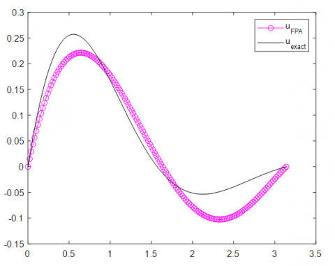
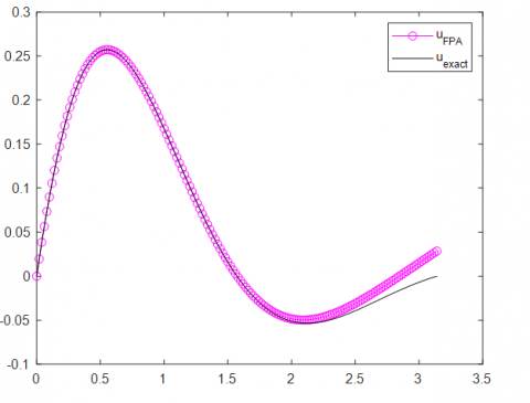
Figures 1 and 2 make a comparison of the approximate solutions $Y_{N(x)}$ given using CMSA for $\mathrm{N}=5$ and $\mathrm{N}=7$ with the exact solution $y_{exact}$.
Table 2 shows the Root Mean Square Error obtained by the approximate solution of the integro-differential Eq. (1), using the Chebyshev Metaheuristic Solver Approach and the general approach introduced in reference [20].
Figure 1. Exact solution against CMSA approximation (first problem for $\mathrm{N}=5$)
Figure 2. Exact solution against CMSA approximation (first problem for $\mathrm{N}=7$)
Table 2. Comparison table of RMSE for the integro differential equation obtained by CMSA and PSO ([20])
|
Optimizer |
RMSE |
| CMSA $N=5$ | $3.14 e-02$ |
| CMSA $N=7$ | $1.05 e-02$ |
| PSO | $1.805 e-01$ |
The results reveal an excellent agreement between the exact and the approximate solutions. The approximation quality enhances visibly as the polynomial degree $N$ augments from 5 to 7, proving the expected convergence comportment of the Chebyshev approximation facilitated by the FPA's coefficient search. The approximate solutions nearly trace the exact curve within the entire domain, especially for $N=7$.
3.2 Second problem; non-Linear Bernoulli boundary value problem
Now, tracking the non-linear Bernoulli equation represented as a boundary value problem:
$y^{\prime \prime}(x)+\left(y^{\prime}(x)\right)^2-2 e^{\{-y(x)\}}=0$
with the boundary conditions $y(0)=0$ and $y(1)=0$, among the interval $[0,1]$.
The exact solution of the suggested problem is:
$y_{exact}(x)=\ln \left(\left(x-\frac{1}{2}\right)^2+\frac{3}{4}\right)$
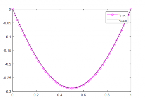
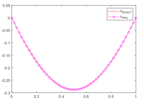
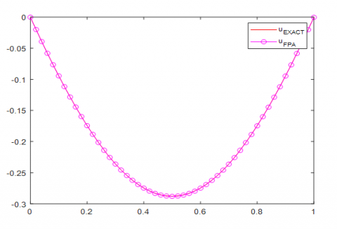
The CMSA was implemented with $N=5,7,9$. FPA parameters were the same as those employed in the first example (see Table 1). Figures 3-5 compare the CMSA approximations against the exact solution for $\mathrm{N}=5, \mathrm{~N}=7$, and $\mathrm{N}=9$, respectively.
The approximate solutions obtained from using CMSA are:
For $\mathrm{N}=5$
$\begin{aligned} & y_5(x)=2.7085 e-16 x^5-0.5403 x^4+1.0805 x^3 +0.4798 x^2-1.0200 x-7.0000 e-06\end{aligned}$
For $\mathrm{N}=7$
$\begin{array}{r}y_7(x)=0.1304 x^7-0.2878 x^6+0.1077 x^5-0.4096 x^4 +0.9883 x^3+0.4854 x^2-1.0146 x\end{array}$
Or,
$\begin{aligned} y_7(x)=-0.00082011 T_0(x)-0.13476 T_1(x)-0.096989 T_2(x)+0.32353 T_3(x) -0.10515 T_4(x)+0.020998 T_5(x)-0.0089923 T_6(x)+0.002038 T_7(x)\end{aligned}$
For $\mathrm{N}=9$
$\begin{aligned} y_9(x)=-0.2689 & x^9+0.5652 x^8+0.3149 x^7-1.3724 x^6+0.6025 x^5-0.0599 x^4+0.7203 x^3+0.4990 x^2-1.0010 x-0.0001\end{aligned}$
Or,
$\begin{array}{rl}y_9(x)=-0.047 & 332 T_0(x)-0.044291 T_1(x) -0.17647 T_2(x)+0.38347 T_3(x) -0.14118 T_4(x)+0.034289 T_5(x) \\ & -0.007565 T_6(x)-0.0045317 T_7(x) \\ & +0.0044153 T_8(x)-0.0010502 T_9(x)\end{array}$
Table 3. Comparison table of RMSE for the non-linear Bernoulli equation obtained by SPMS and PSO ([20])
|
Optimizer |
RMSE |
| CMSA $N=5$ | $1.9 e-03$ |
| CMSA $N=7$ | $1.1 e-03$ |
| CMSA $N=9$ | $2.8144 e-04$ |
| PSO $N=5$ | $3.0503 e-04$ |
Table 3 shows the Root Mean Square Error obtained by the approximate solution of the non-linear Bernoulli equation (second problem), using the Chebyshev metaheuristic solver and the general approach introduced in reference [20].
Figure 3. Exact solution against CMSA approximation (second problem for $\mathrm{N}=5$)
Figure 4. Exact solution against CMSA approximation (second problem for $\mathrm{N}=7$)
Figure 5. Exact solution against CMSA approximation (second problem for $\mathrm{N}=9$)
High degree of agreement is observed for all tested degrees $N$. Even with $N=5$, the shape of the exact solution has been well captured by the approximation. As $N$ augments to 7 and 9, the approximate solution come to be graphically indistinguishable from the exact solution, showcasing the method's ability to handle non-linearities and boundary conditions efficiently. The fast convergence suggests that the integration of Chebyshev polynomials and FPA optimization navigates with success the solution space to obtain highly accurate coefficient sets.
This paper presented a Chebyshev Metaheuristic Solver Approach (CMSA), a hybrid computational strategy for solving differential equations. By formulating the approximate solution using Chebyshev polynomials and using the Flower Pollination Algorithm to approximate the coefficients based on the minimization of the equation residual and boundary condition deviations, we instituted a versatile framework valid to various DE types.
The experimental results found for both linear integro-differential and non-linear boundary value problems prove the efficiency and accuracy of the suggested approach. The CMSA leaded with success approximations that converge fast towards the exact solutions as the degree of the polynomial expansion augments. The approach integrates the power of spectral approximation with the robust search abilities of metaheuristics.
Future studies could be done:
|
$a_j$ |
Vector of Chebyshev polynomial coefficients |
|
$a_{ {best }}$ |
Best coefficient vector found by FPA |
|
$a_{ {cand }}$ |
Candidate coefficient vector in FPA |
|
$a^j, a^k$ |
Randomly chosen coefficient vectors from population in FPA |
|
$a^t$ |
Coefficient vector at FPA iteration $t$ |
|
$C_i(y)$ |
$i$ -th boundary or initial condition operator |
|
$d_i$ |
Specified value for the $i$ -th boundary or initial condition |
|
$f$ |
Function defining the differential equation |
|
$H$ |
Heaviside step function |
|
$k$ |
Order of the highest derivative in the differential equation |
|
$L$ |
Step size in FPA global pollination, drawn from Lévy distribution |
|
$L b$ |
Lower bound for coefficient values in FPA search space |
|
$M$ |
Number of collocation points |
|
MaxIter |
Maximum number of iterations for FPA |
|
$N$ |
Degree of the Chebyshev polynomial approximation |
|
$n_{ {pop }}$ |
Population size in FPA |
|
objf |
Objective function to be minimized |
|
$p$ |
Switching probability in FPA |
|
$R\left(x ; a_i\right)$ |
Residual function of the DE using the approximate solution |
|
ResidualError |
Sum of squared residuals over collocation points |
|
$r$ |
Random number uniformly distributed in [0,1) for FPA logic |
|
$T_j$ |
Chebyshev polynomial of the first kind of degree $j$ |
|
$t$ |
Iteration counter in FPA |
|
$U$ |
Random number drawn from a uniform distribution U (0,1) for FPA local pollination |
|
$U b$ |
Upper bound for coefficient values in FPA search space |
|
$w_i$ |
Weighting factor for the $i$-th condition penalty |
|
$x$ |
Independent variable |
|
$x_0, x_n$ |
Start and end points of the domain of interest |
|
$x_p$ |
$p$-th collocation point |
|
$Y_N(x)$ |
Approximate solution to the differential equation using $N$ -degree polynomial |
|
$y(x)$ |
General or exact solution to the differential equation |
|
$y^{(k)}(x)$ |
k-th derivative of $y(x)$ with respect to x |
|
$y_{{exact }}(x)$ |
Known exact solution for benchmark problems |
|
Subscripts and Superscripts |
|
|
$0$ |
Initial value |
|
best |
The best solution found so far |
|
cand |
A candidate solution |
|
exact |
An exact solution |
|
$i$ |
Boundary/initial conditions or general counting |
|
$j, k$ |
Polynomial terms or solutions in FPA |
|
$N$ |
Degree of polynomial approximation |
|
$n$ |
Final value |
|
$p$ |
Collocation points |
|
$t$ |
Iteration number |
|
$(k)$ |
Order of differentiation |
[1] Boyce, W.E., DiPrima, R.C., Coombes, K.R., Hunt, B.R., Lipsman, R.L. (1997). Elementary differential equations and boundary value problems, 6th ed, J. Wiley Sons, New York. https://www.amazon.com/Elementary-Differential-Equations-Boundary-Mathematica/dp/0471282928.
[2] Shen, J., Tang, T., Wang, L.L. (2011). Spectral methods: Algorithms, analysis and applications, Vol. 41. Springer Science & Business Media.
[3] Boussaïd, I., Lepagnot, J., Siarry, P. (2013). A survey on optimization metaheuristics. Information Sciences, 237: 82-117. https://doi.org/10.1016/j.ins.2013.02.041
[4] Črepinšek, M., Liu, S.H., Mernik, M. (2013). Exploration and exploitation in evolutionary algorithms: A survey. ACM Computing Surveys (CSUR), 45(3): 1-33. https://doi.org/10.1145/2480741.2480752
[5] Yang, X.S., Karamanoglu, M. (2020). Nature-inspired computation and swarm intelligence: A state-of-the-art overview. Nature-Inspired Computation and Swarm Intelligence, Algorithm Academic Press, 3-18. https://doi.org/10.1016/B978-0-12-819714-1.00010-5
[6] Holland, J.H. (1984). Genetic algorithms and adaptation. Adaptive Control of Ill-Defined Systems, Springer, Boston, MA., 16: 317-333. https://doi.org/10.1007/978-1-4684-8941-5_21
[7] Kennedy, J., Eberhart, R. (1995). Particle swarm optimization. In Proceedings of The IEEE International Conference on Neural Networks, Perth, WA, Australia, pp. 1942-1948. https://doi.org/10.1109/ICNN.1995.488968
[8] Karaboga, D. (2010). Artificial bee colony algorithm. Scholarpedia, 5(3): 6915. http://doi.org/10.4249/scholarpedia.6915
[9] Yang, X.S. (2010) Firefly algorithm, an introduction with metaheuristic applications. Engineering Optimization: An Introduction with Metaheuristic Applications, 221-230. https://doi.org/10.1002/9780470640425.ch17
[10] Yang, X.S. (2010). Nature-inspired metaheuristic algorithms. Luniver Press.
[11] Gandomi, A.H., Yang, X.S., Alavi, A.H. (2013). Cuckoo search algorithm: A metaheuristic approach to solve structural optimization problems. Engineering with Computers, 29(2): 17-35. https://doi.org/10.1007/s00366-011-0241-y
[12] Mirjalili, S., Lewis, A. (2016). The whale optimization algorithm. Advances in Engineering Software, 95: 51-67. https://doi.org/10.1016/j.advengsoft.2016.01.008
[13] Sulaiman, M.H., Mustaffa, Z., Saari, M.M., Daniyal, H. (2020). Barnacles mating optimizer: A new bio-inspired algorithm for solving engineering optimization problems. Engineering Applications of Artificial Intelligence, 87: 103330. https://doi.org/10.1016/j.engappai.2019.103330
[14] Zhao, S., Zhang, T., Ma, S., Chen, M. (2022). Dandelion Optimizer: A nature-inspired metaheuristic algorithm for engineering applications. Engineering Applications of Artificial Intelligence, 114: 105075. https://doi.org/10.1016/j.engappai.2022.105075
[15] Agushaka, J.O., Ezugwu, A.E., Abualigah, L. (2022). Dwarf mongoose optimization algorithm. Computer Methods in Applied Mechanics and Engineering, 391: 114570. https://doi.org/10.1016/j.cma.2022.114570
[16] Ahmadkhanpour, F., Kheiri, H., Azarmir, N., Khiyabani, F.M. (2025). Solving initial value problems using multilayer perceptron artificial neural networks. Computational Methods for Differential Equations, 13(1): 13-24. 10.22034/cmde.2024.58774.2486
[17] Lu, L., Meng, X., Mao, Z., Karniadakis, G.E. (2021). DeepXDE: A deep learning library for solving differential equations. Society of Industrial and Applied Mathematics Review, 63(1): 208-228. https://doi.org/10.1137/19M1274067
[18] Parand, K., Aghaei, A.A., Kiani, S., Zadeh, T.I., Khosravi, Z. (2024). A neural network approach for solving nonlinear differential equations of Lane-Emden type. Engineering with Computers, 40(2): 953-969. https://doi.org/10.1007/s00366-023-01836-5
[19] Yang, X.S. (2012). Flower pollination algorithm for global optimization. In International Conference on Unconventional Computing and Natural Computation. Berlin, Heidelberg: Springer Berlin Heidelberg, pp. 240-249. https://doi.org/10.1007/978-3-642-32894-7_27
[20] Babaei, M. (2013). A general approach to approximate solutions of nonlinear differential equations using particle swarm optimization. Applied Soft Computing, 13(7): 3354-3365. https://doi.org/10.1016/j.asoc.2013.02.005