Abderraouf Seniguer*![]() | Abdelhamid Iratni
| Abdelhamid Iratni![]() | Mustapha Aouache
| Mustapha Aouache![]() | Hadja Yakoubi
| Hadja Yakoubi![]() | Haithem Mekhermeche
| Haithem Mekhermeche![]()
© 2025 The authors. This article is published by IIETA and is licensed under the CC BY 4.0 license (http://creativecommons.org/licenses/by/4.0/).
OPEN ACCESS
Adequate indoor lighting is essential for ensuring visual comfort, energy efficiency, and compliance with architectural standards. This study presents a novel smartphone-based platform for real-time illuminance estimation and visual mapping, that leverages a lightweight machine learning model. The application utilizes the smartphone’s built-in camera to capture images of the scenes and performs illuminance prediction for each patch of the image using a trained regression model, offering a cost-effective alternative to physical lux meter grid. The mobile application generates a color-coded heat maps that visualize the spatial distribution of illuminance and do the assessment of its compliance with an established lighting norm. The advantages of the proposed system include its affordability, portability, and prediction accuracy enabled by the machine learning model trained on image intensity features. Experimental tests in a controlled indoor setting demonstrate high prediction accuracy and low computational requirements, confirming the platform’s suitability for use in real-word applications. The tool enables effective and precise analysis of light and is hence usable in architectural diagnostics, energy audits, and spatial design optimization. In addition, the user-friendly interface benefits both professional and non-professional users, facilitating real-time adjustment and optimization of indoor lighting.
energy efficiency, illuminance estimation, indoor lighting design, lighting compliance, machine learning regression, smartphone application
The push for smarter and greener buildings has made indoor lighting a central aspect of energy-efficient architectural design. According to the international energy agency, lighting represents a major component of energy use in residential and commercial buildings account for as much as 15% of worldwide electricity consumption [1]. Ensuring both efficient and comfortable lighting conditions is no longer a matter of convenience; it is a fundamental requirement for environmental sustainability and occupant well-being [2]. Traditional illuminance measurement methods, such as handheld lux meters or wall-mounted ambient light sensors, often fall short when deployed in practical, large-scale applications. First, these tools provide only single-point measurements, failing to capture spatial variability in lighting conditions, which is crucial for identifying under- or over-illuminated zones. This lack of spatial resolution makes them impractical for environments like classrooms, offices, or retail spaces where lighting uniformity directly affects comfort and productivity. Second, the requirement of manual operation, precise sensor placement, and professional calibration limits their accessibility for non-expert users. Additionally, high-quality lux meters are typically expensive and may not be feasible for widespread deployment in low-resource settings. These limitations emphasize the need for cost-effective, user-friendly solutions that offer spatially-resolved, real-time feedback without relying on specialized instrumentation or trained personnel [3].
Several recent studies have explored the capabilities of image processing techniques to overcome the difficulties faced by the traditional lux meter method. Kamath et al. [4] presented the analysis of illuminance on work plane prediction from low dynamic range, raw image data. While their methodology demonstrates that images from cameras can be utilized as a stand-in for lux measurements, it is restricted to controlled testing environments and lacks the ability to produce visual illumination maps. Moreover, Abderraouf et al. [5] designed a vision-based indoor lighting estimation method primarily geared toward daylight harvesting, using image processing to classify ambient lighting conditions, However, their approach did not integrate predictive modelling or user feedback mechanisms, exhibited limited accuracy in illuminance prediction, and lacked the ability to produce interpretable illuminance overlays.
Kruisselbrink et al. [6] proposed a custom-built device for luminance distribution measurement using High Dynamic Range (HDR) imaging method, a widely used technique in photography which is based on the principal of capturing a wider dynamic range. Their system demonstrated good indoor light estimation accuracy. Nonetheless, it was non-portable, required dedicated hardware, had high computational demands, and needed time-consuming calibration by trained personnel. Similarly, Bishop and Chase [7], introduced a low-cost luminance imaging device using HDR technique with goal of minimizing calibration needs. While economical, this application also relies on external imaging components, and lacked the real-time, lightweight capabilities required for mobile usage.
In addition to image-processing-based strategies, several learning-based techniques have demonstrated high potential in indoor illumination estimation. For example, Wang et al. [8] proposed CGLight, which combines a ConvMixer backbone with a GauGAN-based image-to-illumination mapping framework, enabling the generation of spatially consistent and realistic lighting predictions. Similarly, in their FHLight model, Wang et al. [9] introduced enhancements in the loss function design to improve model robustness across diverse lighting distributions and indoor geometries. Zhao et al. [10] presented SGformer, a transformer-based architecture that incorporates both global context and local spatial cues through self-attention mechanisms, allowing it to accurately estimate spherical lighting parameters from single RGB images. While these methods achieve state-of-the-art accuracy in complex visual scenes, their reliance on deep feature hierarchies, large-scale annotated datasets, and GPU acceleration limits their practicality for mobile deployment. In contrast, our approach adopts a lightweight machine learning framework tailored for on-device inference, achieving a favorable trade-off between accuracy, interpretability, and computational efficiency, particularly suited for real-time illuminance analysis on smartphones.
Some researchers have also investigated the utility of smartphone-embedded ambient light sensors (ALS) for lux estimation and indoor localization tasks [11]. Although such sensors are useful for low-power applications, they typically provide single-point measurements with limited accuracy. In particular, Gutierrez-Martinez et al. [11] reported an absolute error when estimating illuminance of close to 10%. In contrast, our camera-based approach, trained via machine learning regressors, achieved a significantly lower error of around 2.4%. Additionally, the use of features extracted from images allows our method to generate spatially dense lighting maps.
This paper introduces an innovative smartphone-based mobile application that take advantage of a high performance lightweight machine learning model for real-time illuminance estimation and visualization. The app utilizes the smartphone’s built-in camera to capture indoor scenes, segments them into localized patches, and estimates illuminance at the patch level using a trained regression model. The predictions are then used to create color-coded heat map overlay, which provides intuitive feedback on spatial lighting distribution. The average illuminance value of the captured scene is then compared with standards set by the Commission on Illumination (CIE) and the Illuminating Engineering Society (IES) to assess whether the current lighting conditions falls under the recommended levels for typical indoor settings or not.
In contrast with the previous studies that rely on static laboratory conditions, external hardware or needs a high computation power our solution is platform-independent, cost-effective, and optimized for practical mobile use. Through the integration of visual feedback and machine learning inference, it facilitates accessible, real-time assessment of indoor lighting, offering value to architects, lighting designers, educators, and facility managers, this study is guided by two core research questions:
·What level of accuracy can be achieved using different machine learning regressors (MLP, Random Forest, Gradient Boosting) when predicting patch-wise illuminance from camera-derived features?
·Can such a system operate efficiently on mobile devices while providing interpretable, standards-based feedback aligned with lighting guidelines?
These questions drive the development, validation, and deployment of the mobile application described herein. This paper proceeds with Section 2, which details the approach used for data collection, model development, and application workflow. Section 3 presents experimental findings and model evaluations conducted under varying real-world lighting scenarios. The paper concludes with key insights and proposed directions for future work.
The system developed in this study represent a real-time indoor illuminance estimation tool that utilizes a smartphone's onboard camera with a trained machine learning model. Illuminance, or the total luminous flux per unit area falling on a surface, is quantified in lux (lx). The mathematical representation of illuminance is given ass:
$E=\frac{\Phi}{A}$ (1)
where, E is illuminance in lux, $\Phi$ is luminous flux in lumens, and A is area in square meters [12]. Illuminance serves as a quantitative metric for assessing the lighting adequacy of a surface, which is crucial for evaluating visual comfort and lighting quality in indoor environments.
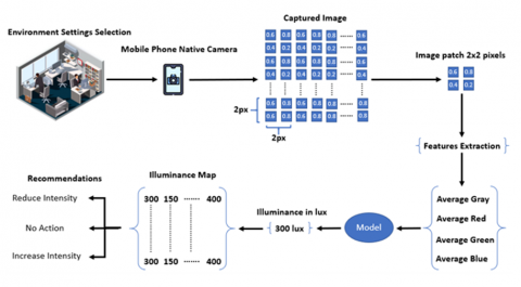
The proposed system consists of four components: (i) a user-friendly mobile application interface, (ii) a machine learning illuminance prediction model, (iii) a heat map visualization module to represent spatial light distribution, and (iv) a recommendation algorithm for assessing compliance with recognized lighting standards. The complete workflow of the platform is illustrated in Figure 1.
Figure 1. Platform architecture and data flow
At the front end, the application enables the user to select a specific indoor environment from a predefined list of use cases (e.g., residential, classroom, retail). Once the analysis is initiated, the smartphone's rear camera activates and captures a frame of the current scene. Images were captured using a Xiaomi Redmi Note 8 smartphone, equipped with a 48MP camera (f/1.8, 1/2.0", 0.8µm) at a 524×324 pixels resolution prior to processing and model training. This resolution was empirically found to offer a balance between spatial detail and computational efficiency and visual aesthetic.
The captured image is subsequently divided into small 2×2 pixel patches, providing a fine-grained assessment of lighting distribution while maintaining low computational overhead. Each patch is analyzed based on the mean intensity values of its red, green, and blue (RGB) channels, which serve as the input features for the illuminance prediction model.
The model selected in our study was implemented using TensorFlow.js that allows machine learning models to make inference locally on the device without the need for external servers which enhances both security and offline accessibility. For each patch, the model estimates the corresponding lux value. These values are then stored into a two-dimensional illuminance matrix which represent the predicted light intensity across the captured scene.
Viridis color map is then used to create a color-coded heat map overlay to depict the spatial distribution of illuminance levels throughout the scene. The overlay is rendered on top of the original image via the use of canvas blending techniques, allowing dynamic, intuitive, and real-time visualization.
Simultaneously, the platform also computes the general average illuminance value of the whole frame and compares it against the recommended lux levels defined for the selected indoor setting. Based on this comparison, the application app categorizes regions as underlit, adequately lit, or overlit, and delivers contextual lighting recommendations to the user.
This methodology enables intuitive interpretation of lighting adequacy by non-expert users, removing the need for specialized instrumentation or technical knowledge. The platform's emphasis on accessibility and real-time responsiveness supports its applicability in diverse settings, including education, healthcare, office, and residential environments.
2.1 Data collection and labelling
To develop a robust and accurate predictive model for real-time indoor illuminance estimation using smartphone imagery, a dedicated dataset was constructed under controlled experimental conditions. The objective was to establish a quantitative relationship between visual features extracted from image patches and their corresponding ground truth illuminance values (in lux), as measured by a calibrated physical sensor.
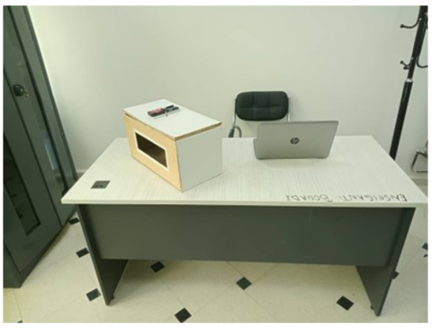
The data acquisition process was carried out in a scaled indoor mock-up environment designed to replicate typical residential and office lighting conditions, as shown in Figure 2. The lighting environment consisted of both natural daylight whose intensity varied over time and artificial lighting provided by a dimmable 5730 white LED strip.
Figure 2. Scaled mock-up for data collection process
The artificial lighting intensity modulated using a potentiometer interfaced with an Arduino microcontroller via Pulse Width Modulation (PWM) signals, enabling precise and continuous control of the lighting output. This setup facilitated the simulation of diverse real-world lighting scenarios across different times of day, enhancing the robustness of the dataset for training and evaluation purposes.
To collect paired data points, a smartphone was mounted in a fixed and stable position to periodically capture images of a predefined target area within the indoor mock-up environment. The image resolution was fixed, and camera parameters including white balance, ISO, exposure, and focus were manually locked to reduce the influence of automatic software enhancements and ensure consistency and reproducibility throughout the dataset.
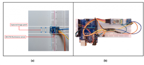
Images were captured at a resolution of 524×324 pixels before patch extraction. Simultaneously, a BH1750 ambient light sensor was placed at the center of the imaged scene and connected to the Arduino platform, the BH1750 is a digital light sensor capable of measuring illuminance from 1 to 65535 lux with an accuracy of ±0.5%, and was chosen for its reliability and ease of integration via the I2C protocol. The complete hardware configuration is illustrated in Figure 3.
Figure 3. Scaled room interior data collection process (a), custom-built illuminance sensor circuit (b)
For each captured image, a synchronized illuminance reading was recorded using timestamp alignment, enabling a precise one-to-one mapping between each image and its respective lux measurement.
To eliminate the effect of surface reflectance and ensure that the lux measurements reflected true light intensity, the scene’s surface was covered with a uniform layer of neutral gray matte material (18% reflectance). This is a widely adopted reference surface in professional photographic and lighting calibration, and it helped minimize bias in RGB values caused by glossy, reflective, or dark absorptive textures, while also reducing specular noise in the captured images.
For each collected image a 2×2 pixel patch was segmented and extracted, a resolution selected to provide a trade-off between spatial granularity and computational efficiency. For each patch, four features extracted and stored for training:
·Mean intensity of the red channel (R_avg).
·Mean intensity of the green channel (G_avg).
·Mean intensity of the blue channel (B_avg).
·The average grayscale intensity (GS_avg).
The grayscale intensity was calculated using the standard luminance transformation, defined as follows:
$G S=0.2989 * R+0.5870 * G+0.1140 * B$ (2)
where, R, G, and B are red, green, and blue channel intensities, respectively.
These four normalized values were normalized to a [0–1] range and used as input to the regression models, while the corresponding illuminance (ILS), measured in lux, by the BH1750 sensor, served as the target output label. Although the lux sensor captures only a single-point reading, the captured scene was carefully composed and uniformly illuminated to ensure that the recorded value accurately represented the lighting condition of the imaged region.
Data acquisition was performed at one-hour intervals throughout an entire calendar year, capturing a wide range of lighting scenarios from low-light conditions in the early morning and high-intensity illumination at midday, to artificially lit environments during the evening.
The final curated dataset comprises 2,650 entries, each representing a distinct 2×2 patch under specific lighting conditions, paired with a corresponding ground-truth illuminance value (in lux), measured using a BH1750 digital light sensor. Each data entry includes R_avg, G_avg, B_avg, GS_avg as features and ILS as target output.
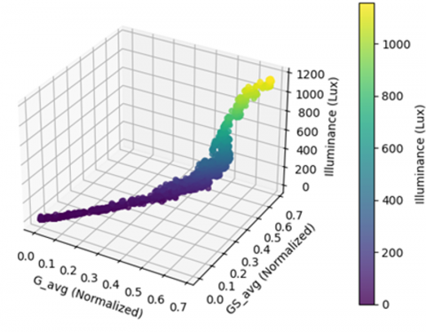
Illuminance values in the dataset span a wide range, from 0 lux to over 1,200 lux, successfully capturing a representative distribution of low, moderate, and high lighting conditions typically encountered in indoor spaces.
To further analyze the internal coherence of the dataset, a 3D scatter plot (Figure 4) was generated to visualize the relationship between G_avg, GS_avg, and ILS. The resulting plot reveals a smooth, monotonically increasing surface, with no evident anomalies, thereby supporting the internal consistency and reliability of the collected dataset.
Figure 4. 3D scatter plot_ G_avg vs GS_avg vs ILS
2.2 Model design and training
The indoor illuminance estimation from image-derived features constitutes a regression task characterized by a continuous output space. The principal objective of this step is to construct predictive models capable of accurately estimating illuminance from low-resolution 2×2 color pixel patches. To achieve this, three machine learning models were selected, trained, and evaluated:
·Multi-Layer Perceptron (MLP) Regressor.
·Random Forest Regressor (RFR).
·Extreme Gradient Boosting (XGBoost) Regressor.
These models were chosen based on their established success in image-based regression tasks, and their ability to model complex nonlinear relationships between input features and target outputs.
2.2.1 Multi-Layer Perceptron regressor
The Multi-Layer Perceptron (MLP) is a fully connected feedforward neural network widely used for regression and classification due to its ability to model nonlinear input-output relationships. It consists of an input layer, one or more hidden layers, and an output layer, where each neuron computes a weighted sum of inputs, adds a bias, and applies an activation function [13]. The operation of a single neuron can be expressed as:
$a^{(l)}=\Phi\left(\sum \omega_{i j}^{(l)} a_j^{(l-1)} b_i^{(l)}\right)$ (3)
where, $a^{(l)}$ is the activation function of the neuron in layer $l$, $\omega_{i j}^{(l)}$ is the weight connecting neuron $j$ in layer $l$-$1$ to neuron $i$ in layer $l$, $b_i^{(l)}$ is the bias term, and $\Phi$ is the activation function, typically the rectified linear unit (ReLU) for hidden layers in modern applications [14].
MLPs are trained using the backpropagation algorithm, which minimizes a loss function via gradient descent. For regression tasks, the Mean Squared Error (MSE) is commonly used and is defined as:
$M S E=\frac{1}{n} \sum_{i-1}^n\left(y_i-\hat{y}_i\right)^2$ (4)
where, $y_i$ is the true illuminance value, $\widehat{y_{\imath}}$ is the predicted value, and n is the total number of samples.
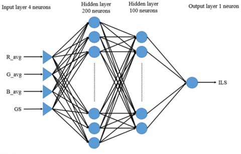
In this study, the MLP consisted of an input layer with four normalized features (R_avg, G_avg, B_avg, GS_avg), two hidden layers (200 and 100 neurons) with ReLU activation, and a single output neuron predicting illuminance (lux). Adam optimizer was used for training due to its adaptive learning rate and efficiency on noisy data [15]. Figure 5 illustrates the architecture, where features are transformed to learn high-level patterns.
Figure 5. MLP architecture for illuminance prediction
The final configuration of the MLP model was obtained through grid search hyperparameter tuning. The optimal parameters are listed in Table 1, and reflect the settings that yielded the best validation performance using k-fold cross-validation.
These hyperparameters were selected based on systematic experimentation and validation results. The MLP Regressor, being a type of feedforward neural network, is capable of learning complex nonlinear relationships between input features and target outputs. Its flexibility makes it suitable for a wide range of problems. However, MLPs are sensitive to the choice of hyperparameters, require more computational resources for training, and may suffer from overfitting with small datasets.
Table 1. The parameters of the MLP model
|
Parameters |
Value |
|
Hidden Layers |
[200, 100] |
|
Activation Function |
ReLU |
|
Solver |
Adam |
|
Learning Rate |
Adaptive |
|
Alpha (L2 regularization) |
0.001 |
|
Loss Function |
MSE |
|
Batch Size |
32 |
2.2.2 Random Forest Regressor
The Random Forest Regressor (RFR) is an ensemble learning method that builds multiple decision trees and averages their outputs, making it effective for nonlinear regression. It enhances generalization and reduces overfitting through bootstrap sampling and random feature selection during training [16]. Each decision tree is trained on a different bootstrap sample (i.e., random sampling with replacement) of the training data. During the construction of each tree, only a random subset of features is considered at each split [17], encouraging decorrelation between trees and enhancing the robustness of the ensemble. The overall prediction of the Random Forest is computed as the average of the predictions made by the individual trees:
$\hat{y}=\frac{1}{T} \sum_{t=1}^T f_t(x)$ (5)
where, $\hat{y}$ is the final prediction, $T$ is the number of decision trees, and $f_t(x)$ is the prediction made by the t -th tree made by for input [18].
Each tree predicts by recursively splitting data based on features to minimize node impurity. For regression, the impurity measure is typically the Mean Squared Error (MSE), defined for node m as:
$M S E_m=\frac{1}{N_M} \sum_{i \in N_m}\left(y_i-\bar{y}\right)^2$ (6)
where, $N_m$ is the set of samples reaching node $m, y_i$ is the target value of sample $i, y_{m}$ is the average target value of the samples in node $m$ [19].
In this study, the Random Forest model was optimized using grid search and k-fold cross-validation, which result the best structure summarized in Table 2.
Table 2. The parameters of the RFR model
|
Parameters |
Value |
|
Number of Trees (n_estimators) |
200 |
|
Maximum Tree Depth |
None |
|
Minimum Samples per Split |
2 |
|
Minimum Samples per Leaf |
1 |
|
Bootstrap Sampling |
Enabled |
|
Splitting Criterion |
MSE |
This configuration allowed the model to learn complex patterns present in the dataset while avoiding overfitting. The number of trees was set to 200 to provide a robust ensemble and to avoid a high increase in training time. Minimum sample constraints used to ensure statistical significance at each node, and by using all four normalized input features in model training allowed the model to take advantage of both color and luminance cues in estimating illuminance.
2.2.3 XGBoost Regressor
The eXtreme Gradient Boosting (XGBoost) Regressor is an advanced gradient boosting algorithm which is characterized by an ameliorated accuracy. It builds an ensemble of decision trees sequentially where each tree tries to correct the errors made by the previous tree by minimizing a loss function via gradient descent this prediction process must sequentially traverse multiple decision trees. Even during inference, this sequential evaluation of hundreds of trees can result in slower prediction speeds compared to simpler models. The model predicts output as a sum of functions, each corresponding a decision tree:
$\hat{y}_i=\sum_{K=1}^K f_K\left(x_i\right), f_K \in \Gamma$ (7)
where, $\Gamma$ is the space of regression trees, $x_i$ is the feature vector for instance $K$ is the number of trees. The optimization objective consists of a loss function measuring prediction error and a regularization term to penalize model complexity:
$L(\Phi)=\sum_{i=1}^n l\left(y_i, \hat{y}_i\right)+\sum_{k=1}^k \Omega\left(f_k\right)$ (8)
with $l$ as the loss function, $\Omega(f)$ as the regulation term where $T$ is the number of leaves in the tree, $w$ are the leaf weights, and $\gamma, \lambda$ regularization parameters, this formulation enables XGBoost to generalize well on unseen data by controlling overfitting [20].
In this study, XGBoost was trained using the normalized features R_avg, G_avg, B_avg, and GS_avg as input, with illuminance (ILS) as the output. Grid search and cross-validation were used to identify the optimal hyperparameters, as shown in Table 3.
Table 3. The parameters of the XGboost estimator
|
Parameters |
Value |
|
Number of Trees |
100 |
|
Maximum Tree Depth |
6 |
|
Learning Rate |
0.1 |
|
Loss Function |
MSE |
|
Regularisation |
L2($\lambda$ =1) |
Every tree in the ensemble, splits the input space into distinct subsets depending on the most informative input attributes. As trees are added sequentially, the model corrects its previous errors iteratively, leading to a robust predictor with the ability to effectively estimate illuminance for different lighting conditions.
2.2.4 Training and validation
In this study, a well-structured and systematic strategy was applied to carry out the training and validation of the three regression models in order to identify the most effective one for practical deployment in real-world lighting assessment tasks. The primary objective was to construct machine learning models capable of predicting illuminance values from features extracted from smartphone-captured indoor images with both high accuracy and strong generalization performance.
Each one of the three models was trained on a preprocessed and normalized dataset comprising statistical features extracted from 2×2 image patches and their corresponding illuminance values (in lux). Training began by randomly splitting the dataset into 80% training and 20% validation subsets, ensuring that models were evaluated on unseen data. To ensure a fair and consistent basis for comparative analysis all models utilized the same training-validation split.
Subsequently, each model underwent hyperparameter tuning via Grid Search Cross-Validation to identify the combination of parameters yielding the optimal performance on the validation set. The tuned parameters for the MLP Regressor model, the tuned are the hidden layer sizes, activation function, the solver, the alpha value, and the learning rate. For the RFR model, the tuned parameters were number of estimators, maximum depth, minimum samples split, and minimum samples leaf. Finally, for XGBoost Regressor the hyperparameters are the number of trees, the maximum tree depth, learning rate, loss function, and the regularization parameters.
To optimize the models hyperparameter Grid Search with k-fold Cross-Validation was performed this process is a robust technique for evaluating parameter combinations and avoiding overfitting. The following hyperparameters were tuned for each model:
·MLP Regressor: number of hidden layers and their sizes, activation function, solver (optimizer), L2, batch size, loss function, and learning rate.
·Random Forest Regressor: number of trees (n_estimators), maximum tree depth, minimum samples required to split a node, and minimum samples per leaf.
·XGBoost Regressor: number of trees, maximum tree depth, learning rate, loss function, and regularization parameter L2.
The process of evaluating the regression models requires robust and interpretable evaluation metrics. In this study we employed three widely accepted indicators to assess performance:
$M A E=\frac{1}{n} \sum_{i=1}^n\left|y_i-\hat{y}_i\right|$ (10)
MAE’s reliance on absolute values makes it less sensitive to outliers than squared-error measures like Mean Squared Error (MSE). In addition to MAE, Root Mean Squared Error (RMSE) was also used, which is defined as:
$R M S E=\sqrt{\frac{1}{n} \sum_{i=1}^n\left(y_i-\hat{y}_i\right)^2}$ (11)
RMSE retains MSE’s sensitivity to large errors while expressing them in the target variable’s units (lux), enhancing interpretability. It effectively highlights significant prediction errors, which are crucial in lighting-sensitive settings like laboratories.
To measure the proportion of variance in the target variable that can be explained by the model, the R² score was used:
$R^2=1-\frac{\sum_{i=1}^n\left(y_i-\hat{y}_i\right)^2}{\sum_{i=1}^n\left(y_i-\bar{y}\right)^2}$ (12)
where, $\bar{y}$ is the mean of the true illuminance values. A perfect model yields $R^2=1$, whereas an $R^2$ close to 0 indicates poor model performance. $R^2$ provides an intuitive measure of model fit and is useful for comparing model generalization on validation data.
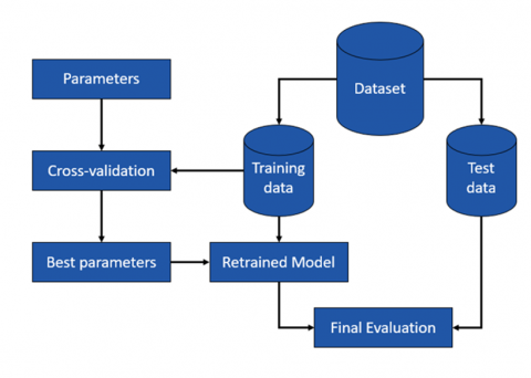
Figure 6 illustrates the training and validation pipeline employed in this study, depicting the sequential process for developing and evaluating the illuminance estimation models.
Figure 6. Training and validation process
The dataset was first split into training and test sets. Using cross-validation on the training data, hyperparameters for the MLP, Random Forest, and XGBoost Regressors were tuned to optimize model fit and generalization.
The best models were then retrained on the full training set and evaluated on the unseen test set. Performance was assessed using MAE, RMSE, and R² to measure accuracy and generalization.
2.3 Mobile app functionality
The lightweight mobile application developed in this study is able to make a real-time illuminance analysis using a trained machine learning model to process camera input, generate an illuminance heatmap, and provide actionable lighting recommendation entirely on-device, without relying on external computation or connectivity.
As shown in Algorithm 1, the app captures an image, divides it into 2×2 patches, and extracts average R, G, B, channels and grayscale intensity from each patch. These normalized inputs are then passed into a TensorFlow.js-based model deployed within the mobile environment, enabling real-time inference for each patch.
The results form a color-coded heatmap overlay on the original image, while the average illuminance is compared against standards for the selected indoor environment.
|
Algorithm 1. Mobile Application workflow. |
|
Input: Live camera feed, selected environment. Output: Illuminance heat map, average lux, lighting recommendation. 1: User selects environment from dropdown menu. 2: Load trained model and initialize rear camera stream. 3: Upon user action ("Scene Analysis"), capture image frame. 4: Divide captured image into 2×2 pixel patches. 7: For each patch: 8: a. Compute normalized R_avg, G_avg, B_avg, and GS_avg. 9: b. Pass input vector [R, G, B, GS] to trained model. 10: c. Predict illuminance (in lux) and assign color from heat map. 11: Render overlay heat map and compute average illuminance value. 12: Retrieve recommended lux range for selected environment. 13: If average_lux < min or > max: 14: a. Display warning with diagnostic message. 15: b. Offer button to show problem areas: 16: - Red overlays for over-illuminated patches. 17: - Blue overlays for under-illuminated patches. 18: Else: 19: a. Display optimal lighting confirmation. 20: Allow user to repeat process or return to camera. |
To determine whether the measured value falls outside or within the acceptable range recommended by CIE and IES associations, Table 4 illustrates the recommended illuminance levels for most possible indoor settings.
Table 4. Recommended lux level
|
Environment |
Recommended Illuminance (lux) |
|
Residential (Living Room) |
100 – 250 |
|
Residential (Bedrooms) |
60 – 100 |
|
Residential (Kitchen) |
300 – 750 |
|
Classroom/office |
300 – 750 |
|
Laboratory |
200 – 500 |
|
Operating Rooms |
300 – 500 |
|
Conference Rooms |
200 – 500 |
|
Display Areas |
750 – 1500 |
The app automatically provides lighting adjustment recommendations based on the computed average illuminance. When the lighting level falls outside the recommended range, a “Highlight Poorly Illuminated Areas” button appears.
Upon activation, the overlay updates to visually mark over-illuminated regions in red and under-illuminated areas in blue, helping users easily identify specific lighting issues.
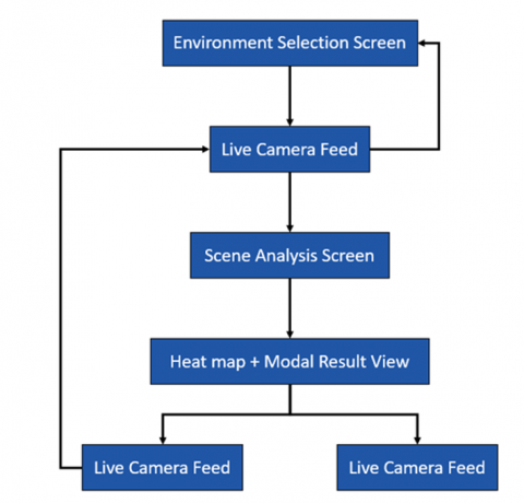
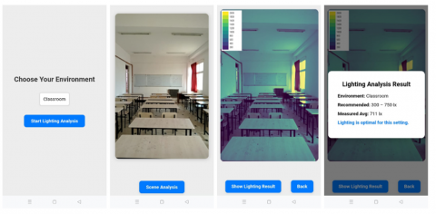
The user interface flow of the mobile application is illustrated in Figure 7 and consists of three main screens. The first screen allows users select an indoor environment (e.g., living room, classroom, retail), each of which is associated to a recommended illuminance range.
Figure 7. User interface flow of the mobile application
After selection, the app moves to the second screen, which streams live video from the smartphone’s rear camera.
Pressing the “Scene Analysis” button freezes the current frame and transitions to the third screen, displaying the analysis overlay and modal recommendations This streamlined flow from environment selection to live preview and finally to interactive feedback ensures an intuitive and efficient user experience.
The primary objective of this study was to develop a robust, mobile-based application for real-time illuminance estimation and spatial mapping application using light-weight machine learning models. To evaluate the performance and viability of the proposed methodology, experiments were conducted on a filtered dataset and through real-world scenario testing using the mobile platform.
This section presents the training results of the three regression models MLP, RFR, and XGBoost based on comprehensive evaluation metrics. Additionally, we evaluate the visual accuracy of the generated illuminance heatmaps, the application’s interactivity, and its responsiveness under diverse lighting conditions.
3.1 Model evaluation and comparison
To evaluate indoor illuminance prediction, three regression models RFR, XGBoost, and MLP were trained using four normalized features extracted from each image patch: R_avg, G_avg, B_avg, and GS_avg. The models were trained and tested on a cleaned dataset with an 80/20 split, with grid search and 5-fold cross-validation employed for hyperparameter tuning. Performance was assessed using Mean Absolute Error (MAE), Root Mean Square Error (RMSE), Coefficient of Determination (R²), and inference time, as summarized in Table 5.
Table 5. Performance comparison of the regression models
|
Model |
MAE |
RMSE |
R² |
Inference Time (s) |
|
RFR |
21.26 |
47.03 lx |
0.9704 |
0.0397 |
|
XGBoost |
23.00 |
50.81 lx |
0.9655 |
0.0021 |
|
MLP |
43.91 |
77.02 lx |
0.9207 |
0.7047 |
As shown in Table 5, the Random Forest Regressor achieved the best balance between accuracy and generalization, with the lowest MAE and RMSE and an R² of 0.9704, demonstrating strong modeling of nonlinear relationships under diverse lighting conditions. Although the XGBoost model exhibited slightly lower accuracy, it significantly outperformed in terms of inference speed (0.0021 seconds per prediction), making it more suitable for time-critical applications on resource-constrained devices. The MLP, despite its theoretical flexibility, underperformed in both accuracy and speed, likely due to the limited input features and small dataset restricting its generalization ability.
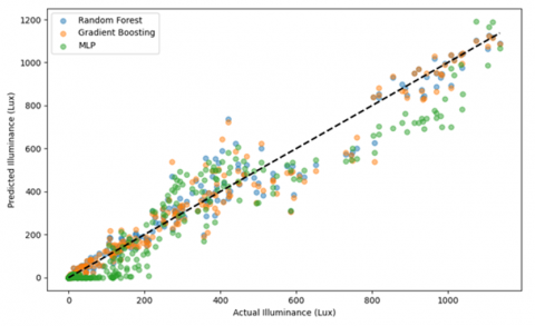
Figure 8 illustrates the predicted versus actual illuminance values for the test set. An ideal model would produce points tightly clustered along the diagonal line. The Random Forest and XGBoost models closely follow this trend, whereas the MLP shows greater variance, with many predictions deviating from the ideal.
Figure 8. Predicted vs. actual illuminance comparison for the three regression models
These findings justify the selection of the Random Forest Regressor for deployment in the mobile application, as its superior accuracy and robustness outweigh the marginal advantage in inference speed offered by XGBoost. Such precision is critical in ensuring reliable compliance with lighting standards and enhancing user comfort in real-world applications.
3.2 Illuminance mapping accuracy and response time analysis
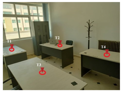
To assess the platform’s real-world, an experiment was conducted to evaluate the spatial accuracy of illuminance mapping and the real-time responsiveness of the mobile application. This study took place in a typical office setting at the Science and Technology Department, Skikda University, Algeria, featuring four desks arranged progressively from a window, creating a natural illumination gradient, as depicted in Figure 9.
Figure 9. Experimental setup for the platform’s real-world evaluation
The setup created a continuous illumination gradient from the window-facing desk (T1) to the farthest desk (T4). Four calibrated digital lux meters were positioned at the center of each desk to establish reliable ground truth measurements. Concurrently, the smartphone app mounted on a fixed tripod to maintain a consistent perspective and distance captured images of the scene under varying lighting conditions.
To introduce lighting variations, artificial light levels were adjusted, and natural light was controlled by opening or closing curtains at different times, enabling testing across diverse lighting conditions. For each setup:
·The smartphone captured an image.
·The model divided the image into non-overlapping 2×2 pixel patches.
·Each patch’s illuminance was predicted using the RFR model.
·Predictions at the four desk centers were compared with lux meter readings.
The predicted values were quantitatively assessed against the ground truth using the Mean Absolute Error Percentage (MAEP), a metric that indicates average prediction deviation as a percentage of true illuminance, providing intuitive insight into visual accuracy. The MAEP was computed using the following equation:
$M E A P=\frac{1}{n} \sum_{i=1}^n\left|\frac{y_i^{ {pred }}-y_i^{ {true }}}{y_i^{ {true }}}\right| \times 100$ (13)
where, $y_i^{{pred }}$ and $y_i^{ {true }}$ represent the predicted and ground truth illuminance values, respectively, and $n$ is the total number of measurement points.
The experiment evaluated multiple lighting scenarios throughout the day, from sunrise to sunset, by capturing a realistic range of indoor illuminance levels typical of office environments. These conditions produced ground truth values in the range of 100–1100 lux, consistent with the standard requirements for office environments.
As illustrated in Figure 10, predicted illuminance values followed actual measurements closely across all four desks. The MAEPs for desks T1, T2, T3, and T4 were 2.22%, 2.72%, 2.38%, and 2.41%, respectively, resulting in a global average MAEP of 2.43%. This low prediction error highlights the system’s ability to generalize across spatial locations and under diverse lighting intensities.
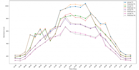
Figure 10. Predicted vs. actual illuminance for tables T1–T4 under varying lighting conditions
In addition to spatial accuracy, the platform's response time was evaluated to assess the feasibility of deploying the solution on mobile devices. Table 6 summarizes the average processing time for each phase of the illuminance analysis pipeline. The end-to-end process from image capture to illuminance mapping and overlay generation required approximately 1.4 seconds, confirming the application’s suitability for real-time use.
Table 6. Processing time for illuminance mapping
|
Process |
Processing Time in [s] |
|
Capturing image |
0.2 |
|
Pre-processing |
0.3 |
|
Illuminance matrix prediction |
0.7 |
|
Uploading results |
0.2 |
|
Total processing time |
1.4 |
To further contextualize the performance of the proposed platform, Table 7 summarizes a comparative analysis of recent studies on indoor illuminance estimation.
Table 7. Comparative analysis of illuminance estimation approaches
|
Study |
Platform Type |
RMSE |
Inference Time (s) |
Notes |
|
Gutierrez-Martinez et al. [11] |
Smartphone ALS |
76 lx |
< 0.01 |
Single-point, non-spatial; limited in low-light environments. |
|
Kamath et al. [4] |
Camera (LDR image) |
79.6 lx |
Not reported |
No visual mapping; tested in controlled conditions only. |
|
Wang et al. [8] |
Deep CNN (CGLight) |
40.2 lx |
~2.3 |
Desktop only; High Latency. |
|
Wang et al. [9] |
Deep CNN (FHLight) |
32.6 lx |
~1.8 |
Requires GPU; not optimized for smartphone deployment. |
|
Zhao et al. [10] |
Transformer (SGFormer) |
30.8 lx |
~2.5 |
Complex; high model size; no spatial heatmap. |
|
Ours |
Smartphone camera |
77.02 lx |
~0.04 |
Real-time, spatial mapping. |
The selected studies include conventional approaches using smartphone ambient light sensors [11], image processing methods [4], and recent learning-based regressors [8, 9] and [10]. While each method presents partial advantage such as cost-effectiveness or algorithmic complexity most suffer from significant limitations in accuracy, spatial resolution, or real-time deployment capability. For example, the smartphone Ambient Light Sensors (ALS) method by Gutierrez-Martinez et al. [11] reports a RMSE of 76 lx, but its single-point measurement nature limits its usability for spatial diagnostics. Likewise, the handcrafted image-based method by Kamath et al. [4] achieved an RMSE of 79.6 lx, but it was tested only in constrained settings using a sophisticated LDR camera sensor and without heatmap generation.
Recent deep learning-based models such as studies [8-10] provide enhanced accuracy on synthetic or benchmark datasets; however, their RMSE still range from 30 lx to 60 lx with inference times unsuitable for mobile applications. In contrast, the proposed Random Forest-based system delivers a MAEP of just 2.43%, corresponding to an RMSE of 47.03 lx, while running in real time on a smartphone and offering spatial illuminance mapping capability.
These findings highlight the effectiveness and efficiency of the proposed platform in delivering real-time, spatially detailed illuminance estimations. The combination of low latency, high spatial fidelity, and minimal error margins makes the system a viable tool for mobile-based lighting diagnostics. Its applications extend to architectural design, smart lighting control, energy auditing, and visual comfort evaluation in both residential and professional environments.
3.3 Application functionality test
To validate the practicality of the proposed mobile illuminance assessment platform, a functionality test was conducted in real-world classroom environment. The objective was to evaluate the application’s responsiveness to typical variations in lighting, including changes in both natural daylight and artificial illumination.
The platform was deployed on a standard Android Xiaomi Redmi Note 8 smartphone and tested in a spacious university classroom at Skikda University, under a variety of lighting conditions ranging from partial daylight to full artificial illumination. For each test session, users executed the entire application workflow, which included:
·Selecting the indoor environment.
·Activating the live video feed.
·Capturing a frame of the scene.
·Generating an illuminance heatmap.
Figure 11 presents a sequence of screenshots representing an optimal lighting scenario. The application accurately detects and maps the indoor light distribution, calculates the average illuminance, and verifies its alignment with the recommended lux range for classrooms (300–750 lx). The resulting heatmap is uniform and consistent, demonstrating the platform's reliability under standard lighting conditions.
Figure 11. Sequence of screenshots for an optimal lighting scenario in classroom setting
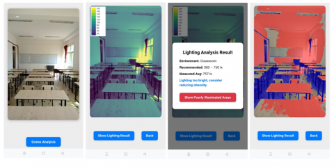
Conversely, Figure 12 shows a contrasting scenario characterized by over-illumination due to excessive natural light exposure.
Figure 12. Sequence of screenshots for an over illuminating lighting scenario in classroom setting
In this case, the application accurately predicted an average illuminance exceeding the upper threshold of the acceptable range. In response, it generated a recommendation to reduce the lighting level. Furthermore, the user utilized the “Show poorly illuminated areas” feature to highlight over-illuminated regions, which were visually marked with red overlays, facilitating easy identification of lighting imbalances.
These two real-case demonstrations confirm the application's effectiveness in delivering actionable feedback through real-time visual analysis, while maintaining consistent user interface behavior and responsiveness under varying conditions. Users noted smooth screen transitions, intuitive interaction flows, and minimal latency during image capture and processing. Overall, the mobile application exhibits strong usability and operational reliability, even in dynamic and fluctuating lighting environments.
3.4 Limitations
While the proposed platform demonstrated promising performance, several limitations must be acknowledged to contextualize its applicability and guide future enhancements.
First, the model’s predictive accuracy is inherently influenced by the hardware characteristics of the smartphone used for image acquisition. Variations in sensor sensitivity, lens quality, and onboard image processing algorithms (such as automatic exposure, white balance correction, or HDR enhancement) can introduce inconsistencies in pixel intensities, thereby affecting the model's generalizability across different devices. Since the current implementation does not incorporate device-specific calibration procedures, variations in camera hardware could lead to discrepancies in illuminance prediction when the application is deployed on heterogeneous smartphones.
Second, the experimental validation was limited to controlled indoor environments specifically, an office and a classroom using a single smartphone model. While these environments are representative of common use cases, they do not encompass the full range of indoor spatial configurations, surface materials, or artificial lighting technologies encountered in real-world applications. Consequently, the model’s scalability and robustness under more diverse conditions, such as residential, commercial, or industrial settings, remain to be validated.
Third, the system's performance may degrade under highly complex or non-uniform lighting scenarios. Conditions involving strong backlighting, mixed color temperature sources, intense reflections, or localized glare can compromise the accuracy of patch-wise illuminance predictions, as such conditions are underrepresented in the current training dataset. Moreover, the system does not currently correct for the non-linear exposure behavior of smartphone cameras in high-dynamic-range scenes, which may further affect luminance estimation in extreme lighting conditions.
Additionally, the absence of a cross-device normalization mechanism poses another limitation. The current approach assumes a uniform camera response function, and does not explicitly account for the wide variability in sensor performance and software tuning across smartphone models. This limits the platform’s ability to deliver consistent results across devices without a prior calibration step.
Finally, although the application performs all computations locally using TensorFlow.js to preserve user privacy and ensure offline functionality, this design choice introduces a non-negligible computational burden. The inference process, which involves predicting illuminance for numerous small patches per frame, can be computationally intensive on smartphones with limited processing capabilities. This may result in latency during real-time operation, particularly on low- to mid-range devices, unless further model optimization or compression techniques are adopted.
This study introduced a low-cost, smartphone-based tool capable of real-time indoor illuminance estimation and mapping, leveraging deep learning and classical machine learning models to support compliance with lighting design standards.
The proposed mobile application enables users to assess lighting conditions visually and numerically, eliminating the need for costly lux meters or specialized instrumentation. Through a platformatic development pipeline encompassing data collection, model training, validation, and integration into a real-world application, we demonstrated that compact devices can provide accurate and spatially-resolved illuminance feedback.
Experimental results showed that among the three tested models Multi-Layer Perceptron, Random Forest Regressor, and Gradient Boosting Regressor; the Random Forest Regressor demonstrated the best trade-off between prediction accuracy (MAE: 21.25, R²: 0.97) and inference speed (≈ 40 ms). Furthermore, Mean Absolute Error Percentage (MAEP) of 2.43% across multiple desk locations in real-world environments, validated the consistency and spatial reliability of the predicted illuminance distribution under varied conditions. The complete application maintained a total processing time of under one second, rendering it suitable for responsive mobile-based lighting analysis. By offering real-time heatmap visualizations and context-aware lighting recommendations within a single portable platform, this application presents new opportunities for intuitive lighting diagnostics in residential, educational, healthcare, and commercial spaces. The user-friendly interface and compatibility with consumer-grade smartphones further enhance its accessibility and scalability.
However, it is important to acknowledge that the platform was only evaluated in a limited range of indoor environments using a single smartphone model. Broader deployment scenarios involving diverse room geometries, surface reflectance, and device-specific camera characteristics should be explored to confirm the model’s robustness and generalizability.
Future work will focus on addressing the current limitations and enhancing the platform's robustness, scalability, and adaptability. A key priority will be the evaluation of system performance across a broader range of real-world indoor environments, including residential, industrial, and commercial settings, each with distinct lighting configurations, surface textures, and spatial geometries. This expanded validation will help assess the model’s generalization capabilities beyond controlled office and classroom scenarios.
To improve cross-device consistency, future versions may incorporate device-specific calibration routines or normalization layers to account for variability in camera hardware and built-in image processing algorithms. In parallel, advanced preprocessing techniques such as high-dynamic-range (HDR) fusion or exposure correction could be explored to better handle scenes with complex or uneven illumination patterns, including glare, shadows, and mixed lighting sources.
From a computational standpoint, optimizing the model for real-time inference on low-end and mid-range smartphones will be essential. This may involve quantization, model pruning, or knowledge distillation to reduce memory and processing demands without compromising accuracy. Furthermore, the integration of lightweight edge computing frameworks could ensure smooth performance while preserving offline functionality.
Finally, future iterations of the system could incorporate temporal illumination tracking and user feedback mechanisms. These enhancements would enable the platform to learn from environmental patterns and user behavior over time, ultimately supporting intelligent daylight harvesting strategies and adaptive lighting control systems that respond dynamically to both spatial and temporal context.
The authors thank the University of Skikda, Skikda, Algeria for providing research facilities and the technical staff members in the Technology Department.
|
RGB |
Red, Green, Blue channel intensities |
|
GS |
Grayscale intensity |
|
ILS MAE |
Illuminance level in lux Mean Absolute Error |
|
RMSE |
Root Mean Square Error |
|
R² |
Coefficient of Determination |
|
MAEP |
Mean Absolute Error Percentage |
|
Subscripts |
|
|
pred |
Predicted illuminance |
|
true |
True (measured) illuminance |
|
lux |
Illuminance in lux units |
[1] International Energy Agency (IEA). (2022). Energy Efficiency 2022. IEA Publications. https://www.iea.org/reports/energy-efficiency-2022.
[2] Garay, R., Chica, J.A., Apraiz, I., Campos, J.M., Tellado, B., Uriarte, A., Sanchez, V. (2015). Energy efficiency achievements in 5 years through experimental research in KUBIK. Energy Procedia, 78: 865-870. https://doi.org/10.1016/j.egypro.2015.11.009
[3] Bergen, T., Young, R. (2018). Fifty years of development of light measurement instrumentation. Lighting Research & Technology, 50(1): 141-153. https://doi.org/10.1177/1477153517731908
[4] Kamath, V., Kurian, C.P., Padiyar, S. (2022). Prediction of illuminance on the work plane using low dynamic unprocessed image data. In 2022 Fourth International Conference on Emerging Research in Electronics, Computer Science and Technology (ICERECT), Mandya, India, pp. 1-5. https://doi.org/10.1109/ICERECT56837.2022.10060471
[5] Abderraouf, S., Aouache, M., Iratni, A., Mekhermeche, H. (2023). Vision-based indoor lighting assessment approach for daylight harvesting. In 2023 International Conference on Advances in Electronics, Control and Communication Systems (ICAECCS), BLIDA, Algeria, pp. 1-6. https://doi.org/10.1109/ICAECCS56710.2023.10104917
[6] Kruisselbrink, T., Aries, M., Rosemann, A. (2017). A practical device for measuring the luminance distribution. International Journal of Sustainable Lighting, 19(1): 75-90. https://doi.org/10.26607/ijsl.v19i1.76
[7] Bishop, D., Chase, J.G. (2023). Development of a low-cost luminance imaging device with minimal equipment calibration procedures for absolute and relative luminance. Buildings, 13(5): 1266. https://doi.org/10.3390/buildings13051266
[8] Wang, Y., Song, S., Zhao, L., Xia, H., Yuan, Z., Zhang, Y. (2024). CGLight: An effective indoor illumination estimation method based on improved ConvMixer and GauGAN. Computers & Graphics, 125: 104122. https://doi.org/10.1016/j.cag.2024.104122
[9] Wang, Y., Wang, A., Song, S., Xie, F., Ma, C., Xu, J., Zhao, L. (2024). FHLight: A novel method of indoor scene illumination estimation using improved loss function. Image and Vision Computing, 152: 105299. https://doi.org/10.1016/j.imavis.2024.105299
[10] Zhao, J., Xue, B., Zhang, M. (2024). SGformer: Boosting transformers for indoor lighting estimation from a single image. Computational Visual Media, 10(4): 671-686. https://doi.org/10.1007/s41095-024-0447-8
[11] Gutierrez-Martinez, J.M., Castillo-Martinez, A., Medina-Merodio, J.A., Aguado-Delgado, J., Martinez-Herraiz, J.J. (2017). Smartphones as a light measurement tool: Case of study. Applied Sciences, 7(6): 616. https://doi.org/10.3390/app7060616
[12] Kabir, K.A., Guha Thakurta, P.K., Kar, S. (2025). An intelligent geographic information system-based framework for energy efficient street lighting. Signal, Image and Video Processing, 19(4): 305. https://doi.org/10.1007/s11760-025-03879-1
[13] LeCun, Y., Bengio, Y., Hinton, G. (2015). Deep learning. Nature, 521(7553): 436-444. https://doi.org/10.1038/nature14539
[14] Villasenor, A. (2023). Machine learning assisted design of mmWave radio frequency circuits. University of California eScholarship. https://escholarship.org/uc/item/5fg6r9pf.
[15] Kingma, D.P., Ba, J. (2014). Adam: A method for stochastic optimization. arXiv preprint, arXiv:1412.6980. https://doi.org/10.48550/arXiv.1412.6980
[16] Breiman, L. (2001). Random forests. Machine Learning, 45: 5-32. https://doi.org/10.1023/A:1010933404324
[17] Dao, N.-N., Pham, Q.-D., Cho, S., Nguyen, N.T. (2024). Intelligence of Things: Technologies and Applications. Springer, Cham. https://doi.org/10.1007/978-3-031-75596-5
[18] Hastie, T., Tibshirani, R., Friedman, J. (2010). The Elements of Statistical Learning: Data Mining, Inference, and Prediction, 2nd ed. Springer, New York. https://doi.org/10.1007/978-0-387-84858-7
[19] Pedregosa, F., Varoquaux, G., Gramfort, A., Michel, V., Thirion, B., Grisel, O., Blondel, M., Prettenhofer, P., Weiss, R., Dubourg, V., Vanderplas, J., Passos, A., Cournapeau, D., Brucher, M., Perrot, M., Duchesnay, E. (2011). Scikit-learn: Machine learning in Python. Journal of Machine Learning Research, 12: 2825-2830. https://dl.acm.org/doi/10.5555/1953048.2078195.
[20] Chen, T., Guestrin, C. (2016). XGBoost: A scalable tree boosting system. In Proceedings of the 22nd ACM SIGKDD International Conference on Knowledge Discovery and Data Mining, pp. 785-794. https://doi.org/10.1145/2939672.2939785