Imadeldin Elsayed Elmutasim![]()
© 2025 The author. This article is published by IIETA and is licensed under the CC BY 4.0 license (http://creativecommons.org/licenses/by/4.0/).
OPEN ACCESS
Wireless propagation is a crucial technology in modern advancements, requiring highly accurate prediction. Path loss propagation is influenced by various parameters that must be accounted for to predict the signal route over the entire distance and refine breakpoint models with precise interference calculations. The breakpoint distance is defined as the point separating two distinct trends of path loss, each following a different path loss exponent. This paper reviews the Fresnel, Perera, and True breakpoints in a dual-slope model reference at 2 GHz, using a fixed exponent of n₁ = 2 before the breakpoint and n₂ = 4 after. It then proposes a distance-adaptive exponent model that considers a steady path by incorporating a flexible exponent based on environmental factors, mitigating the abrupt change in path loss exponent at breakpoints observed in the dual-slope model, which leads to discontinuities. The comparison results under similar conditions demonstrate that both models perform similarly over short distances of up to 100 meters, while the dual-slope model is more suitable for distances of up to 1 km. However, due to its stability and consistency, the distance-adaptive exponent model is more appropriate for longer distances. Validation using RMSE, followed by comparative analysis, confirms that our model offers higher stability in interference scenarios. These findings will assist researchers and wireless designers in predicting and selecting the most accurate and effective propagation model.
wireless technology, dual slope, signal propagation, breakpoint, path loss, two ray model
Wireless communication plays a crucial role in modern technology, enabling high-speed data transfer for applications such as 5G, IoT, and smart city infrastructure. One fundamental challenge while designing wireless networks is accurately modeling signal propagation, which directly impacts network planning, interference management, and coverage optimization. Ideally, path loss models are essential in predicting the attenuation of transmitted signals over distance and are widely used in radio wave propagation studies.
Positioning strategies relying on measured signal strength depend greatly on the precision of RF estimations regarding received power [1-5]. These demands have led researchers in RF prediction to re-evaluate the criteria and precision of current breakpoint location and path loss estimation [6, 7].
Moreover, despite the dramatic expansion of wireless cellular communication networks over the past two decades, they continue to face increasing interference, which degrades service quality. This interference arises from suboptimal cellular network design and inadequate optimization, primarily due to the absence of highly accurate propagation models [8]. No RF path loss model can precisely predict signal intensity, as each model has specific validity constraints and is tailored to particular RF scenarios. To enhance their applicability to real-world RF propagation conditions without causing environmental disruptions, it is vital to understand their rationality ranges and apply necessary correction factors [9, 10].
Traditionally, path loss models fall into two categories: single-slope models, like Free-Space Path Loss, and dual-slope models, which adjust the path loss exponent at a defined breakpoint. The Dual-Slope Path Loss Model provides a more realistic representation of signal attenuation by considering two distinct propagation regions. The first region, before the breakpoint, is dominated by free-space propagation, where the path loss exponent is approximately n1 = 2. Beyond the breakpoint, additional factors such as ground reflection, diffraction, and obstructions contribute to increased signal attenuation, resulting in a higher path loss exponent of n2 = 4, as noted in reference [11].
In contrast, the traditional Dual-Slope Model suffers from abrupt changes in the path loss exponent at the breakpoint, which can lead to discontinuities in signal prediction. This can introduce significant errors, especially in urban and suburban environments, where signal behavior is influenced by multipath effects, terrain variations, and environmental clutter [8, 12]. Researches like Feuerstein et al. [12] and Elmutasim and Mohd [13] define the breakpoint as the point at which the Fresnel zone starts interfering with the ground, while Perera et al. [14] demonstrated that this model exhibits significant discrepancies when assessed against various measurement campaign findings.
Researchers have developed empirical refinement models, such as the Perera breakpoint, which adjusts the breakpoint distance to match suburban and urban propagation data better [15, 16]. However, this approach still uses fixed exponents before and after the breakpoint rather than responding to environmental variability. Other wireless communication design models include standard models such as 3GPP and WINNER II. Such models use environment-specific parameters and empirical exponents; however, they are rigid and do not allow for smooth changes in exponents. Their breakpoint lengths are frequency-dependent and lack physical [17-19]. Another aspect that recent studies have examined is the use of machine learning (ML) models for path loss prediction, which include neural networks and regression trees. These models frequently outperform traditional equations in site-specific deployments; however, they necessitate large, labelled datasets and function as black boxes, which limits their interpretability and portability [20, 21].
To overcome these limitations, we propose distance-adaptive exponent (DAE) model as an adjustable model, where the path loss exponent n varies continuously with distance rather than switching abruptly at a predefined breakpoint. The key contributions of this study are as follows:
• Proposal of DAE model that dynamically adapts the path loss exponent as a function of distance.
• Integration of multiple breakpoints (Fresnel, Perera, and True breakpoints) to refine transition regions between free-space propagation and multipath-dominated environments.
• Comparison of traditional vs. distance-adaptive exponent (DAE) model, highlighting improvements in accuracy and continuity.
• Validation through MATLAB simulations, demonstrating reduced error in path loss prediction.
Breakpoints in wireless propagation modelling describe distances at which signal attenuation changes according to physical or environmental variables. The proposed DAE model incorporates three critical breakpoints: Fresnel, Perera, and True. Each breakpoint is designed to reflect a logical change in propagation behaviour, allowing the model to simulate real-world signal behaviour more accurately in both urban and rural settings.
The Fresnel breakpoint is the crucial distance at which the direct and first-order ground-reflected paths start to interact. It is derived from physical optics and commonly utilized in the Two-Ray Ground Reflection Model, as follows: $d_f=\frac{2 h_t h_r}{\lambda}$, where $h_t$ height of the transmitter, $h_r$ height of the receiver, and $\lambda$ is the wavelength [13]. However, in such a scenario, the breakpoint represents the point beyond which ground reflection and diffraction begin to dominate, and the path loss increases faster than in free-space conditions. The Perera breakpoint $d_p=\frac{4 h_t h_r}{\lambda}$, on the other hand, is an empirical variation of the Fresnel breakpoint. It was initially designed to better suit urban and suburban propagation conditions. It alters the original formulation by adding a greater multiplier. The such breakpoint recognizes the additional complexity of multipath effects, signal dispersion from surrounding buildings, and more aggressive path loss over the theoretical Fresnel distance [12-14]. The literature has used it to provide a more realistic upper limit for free-space propagation in constructed environments. Whereas the third option, known as a True breakpoint, is suggested as a tunable or calibrated distance derived from either measurement data or simulation optimization. It is defined as a scaled version of the Perera distance: $d_T=\alpha \cdot d_p$, where $\alpha$ is an adjustment coefficient that can be tuned based on real-world measurement data or model calibration.
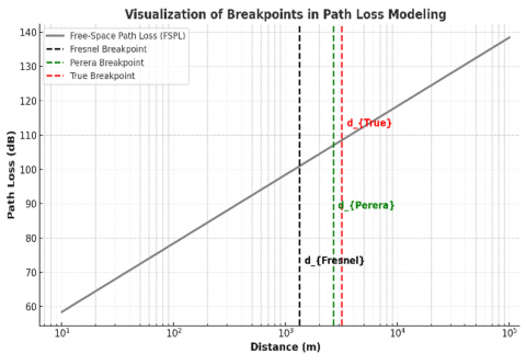
Utilizing these three breakpoints within the adaptive path loss exponent model facilitates segmentation of propagation behaviour over long distances, decreased modelling error, especially near transition zones, and offer capability to represent both ideal theoretical behaviour (Fresnel) and real-world environmental effects (Perera and True) [12-14]. Figure 1 illustrates Free-Space Path Loss (FSPL) along with superimposed Fresnel, Perera, and True breakpoint distances. These thresholds signify transition zones in propagation where the signal's attenuation characteristics alter due to ground reflection, environmental factors, or empirical adjustments.
Figure 1. FSPL with breakpoints in the propagation path
While the proposed model utilizes Fresnel, Perera, and True breakpoints, various other breakpoint models could be introduced in the literature to define path loss transitions, particularly for urban, rural, and mixed environments. These encompass 3GPP UMi and UMa Breakpoints which is defines breakpoints differently for Urban Micro (UMi) and Urban Macro (UMa) environments. For UMa, for instance, $d_{B p 3 G P P}=\frac{2 \pi f_c h_t h_r}{\mathrm{c}}$ which is limited to 3GPP environment definitions, lacks flexibility across topologies and based on the frequency; in addition, the such model does not model exponent as a function of distance; hence causes sharp transitions according to the research [17]. Similar to WINNER II channel models, the breakpoint distance is defined by $d_{{BpWINNER }}=\frac{4 f_c h_t h_r}{\mathrm{c}}$ which is frequency-coupled as well, less intuitive for geometric based on the study [18]. Table 1 shows the comparison of various breakpoints modes specifications using physical basis, tunable possibility, suitability for exponent adaptation, and general model flexibility.
Table 1 clearly illustrates which breakpoint modes are flexible and suitable for adaptive exponent. While these models could evolve into powerful machine learning applications for various purposes, the paper concentrates on interpretable, tunable models appropriate for real-time and wide-area deployment.
Table 1. Breakpoints comparison
|
Breakpoint Type |
Physical Basis |
Tunable |
Suitable for Adaptive Exponent |
Flexibility |
|
Fresnel |
Yes |
No |
Yes |
Low |
|
Perera |
Empirical |
Partly |
Yes |
Medium |
|
True |
Calibrated |
Yes |
Yes |
High |
|
3GPP/ UMa/ UMi |
Empirical/ Frequency based |
No |
No |
Medium |
|
WINNER II |
Frequency-bound |
No |
No |
Low |
Many measurement efforts have confirmed that signal intensity in line-of-sight (LOS) propagation often adheres to the dual-slope attenuation model. The strength of the received signal decreases due to exponential attenuation both prior to and beyond the breakpoint distances, respectively. This dual-slope attenuation model is represented as [22]:
$P L(d)=\left\{\begin{array}{l}P L_1, d \leq d p \\ P L_2, d \geq d p\end{array}\right.$ (1)
where, $P L_1$ and $P L_2$ represent the path loss values before and after the breakpoint location, respectively. d denotes the link separating the transmitter and receiver, while $dp$ is the breakpoint distance that isolate the two slopes.
The conceptual breakpoint distance models rely on the two-ray propagation path loss framework [23, 24], which has been validated through various RF measurement studies. This model describes signal strength, including both direct and reflected waves [25]:
$H(f)=\left|A_t A_r e^{j k d_1}+\Gamma A_t A_r e^{-j k d_2}\right|$ (2)
where, $H(f)$ represents the two-ray path loss model, $A_t$ and $A_r$ are the antenna gains at the transmitter and receiver, respectively, $d_1$ and $d_2$ denote the travelling distances of the direct and reflected beams, respectively, $\Gamma$ is the Fresnel reflection coefficient, while $k$ is the wave factor and equal to 2π/λ.
While according to the study [6], the pathloss could be given by:
$P L=10 \log _{10}\left(\frac{|H(f)|^2}{P_t}\right)$ (3)
where, $P_t$ is transmitted power.
The suggested Perera's breakpoint distance framework, derived by equating the two approximations based on the study [26], is expressed as follows:
$d_{b r k}=8.41 \cdot \frac{h_t h_r}{\lambda}$ (4)
Clearly in Eq. (4) the model predicts $d_{b r k}$ to be more than estimated using the most commonly referenced model introduced in references [8, 12, 13], which can be expressed as $\frac{4 h_t h_r}{\lambda}$. To thoroughly investigate the forecasting precision of Perera's breakpoint distance model, we will compare its effectiveness relative to its underlying framework, the two-ray model. According to studies [24, 26], the communication function of a two-ray radio channel is expressed as follows:
$\begin{aligned} & H_{V, H}=f_t^{V, H}\left(\theta_d^t, \phi_d^t\right) f_r^{V, H}\left(\theta_d^r, \phi_d^r\right) \frac{\lambda}{4 \pi r_d} e^{-j k r_d} \\ & +f_t^{V, H}\left(\theta_g^t, \phi_g^t\right) f_r^{V, H}\left(\theta_g^r, \phi_g^r\right) R_{V, H} \frac{\lambda}{4 \pi r_g} e^{-j k r_g}\end{aligned}$ (5)
where, $f_r^{V, H}(\because)$ and $f_t^{V, H}(\because)$ are receiver and far-field amplitude distributions of the antenna radiation patterns for vertical and horizontal polarizations,, respectively; $\theta_i^{t, r}, \phi_i^{t, r}$ are the transmitter and receiver ray i’s elevation and azimuth angles (direct or reflected), respectively; $r_g$ and $r_d$ denote the propagation distances of the direct and ground (or water) reflected paths, respectively; $k$ is the wave number $\left(k=\frac{2 \pi}{\lambda}\right)$; and $\lambda$ wavelength corresponding to the operating frequency.
Nevertheless, Perera’s model is derivative from the two-ray path loss model and predicts the breakpoint distance $d p$ as:
$d p=\frac{4 h_t h_r}{\lambda}$ (6)
where, $h_t$ and $h_r$ heights of transmitter and receiver antenna, and $\lambda$ is the wavelength of operating frequency.
However, the study [26] introduces a correction term of Perera’s model as:
$Corrected _{d p}=8.41 \cdot \frac{h_t h_r}{\lambda}+C$ (7)
where, $C$ is the correction term given by:
$C=f_1\left(h_r\right)+f_2\left(h_r\right) \frac{h_t}{\lambda}$ (8)
The formulations of $f_1\left(h_r\right)$ and $f_2\left(h_r\right)$ are given in the research [26].
Consequently, our paper’s contribution to improving the dual-slope path loss model by introducing distance-adaptive exponent (DAE) model exponent instead of fixed values. This refinement enables the model to dynamically adjust depending on the link distance between the transmitter and the receiver. Eq. (9) explained the comprehensive concept contribution:
$n(d)=n_1+\gamma \cdot \log _{10}(d)$ (9)
where, $n_1$ is the free-space baseline (typically 2), and $\gamma$ is a tuning parameter reflecting environment dynamics that can clarify $\gamma$ can be empirically related to environmental factors. Thus, the fixed exponent $n_1=2$ which is before breakpoint and $n_2=4$ after the breakpoint, leaded to defined adjustable exponent as:
$n_{D A E}=2+\Upsilon \cdot \log _{10}(d)$ (10)
where, $n_{D A E}$ is the distance-dependent path loss exponent, $\Upsilon$ works as a tunning factor to control the rate of change depends on environment for example in urban = 0.1 up to 0.8 and in rural = 0.05 according to the research [27], whereas $d$ considers the link distance between transmitter and receiver antenna.
Eq. (10) increases the path loss exponent gradually instead of making an abrupt jump from n1 = 2 to n2 = 4, which provides a more realistic transition between different propagation conditions. The idea for this contribution arose to avoid the abrupt switch from traditional models while also providing a smooth transition between different distances, more accurately reflecting real-world propagation. In other words, the approach offers customizable advantage via offering different $\Upsilon$ that allows adjustments for urban, suburban, and rural areas.
This segment showcases simulation results of breakpoint distance in different models using the parameters in Table 2.
Table 2. The significant parameters in the simulation
|
Simulation |
|
|
Parameters |
Values |
|
Frequency |
2 GHz |
|
Transmitter Height |
20 m |
|
Receiver Height |
5 m |
|
Antenna Height |
2 meters |
|
d _Fresnel |
$\frac{2 h_t h_r}{\lambda}$ |
|
d _Perera |
$\frac{4 h_t h_r}{\lambda}$ |
|
d _True |
d_Perera × 1.2 |
|
Path loss exponents |
$n_1$=2 before breakpoint, $n_2$=4 after breakpoint, and $n_{ {adjustable }}=2+\Upsilon \cdot \log _{10}(d)$ |
The simulation setting is consistent with realistic setups found in scenarios. Both LTE and early 5G rollouts often use a 2 GHz carrier frequency, a 20-meter base station height, and a 5-meter receiver height, particularly in suburban or highway installations. As a result, the suggested model is both theoretically sound and relevant to real-world applications such as cell design, handover margin optimization, and interference modelling.
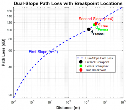
Figure 2. Breakpoint distance in Fresnel, Perera, and True in dual slope path loss
While the Figure 2 describes the dual-slope path loss incorporate with Fresnel, Perera, and True breakpoints. The traditional Dual-Slope model exhibits a sudden change in the path loss exponent at breakpoints, leading to discontinuities.
The models' breakpoints distance using 2 GHz is located from 1 km up to 6 km, while to demonstrate the concept, the investigation was conducted using 7, 10, and 18 GHz to explain the influences, as shown in Figures 3, 4, and 5.
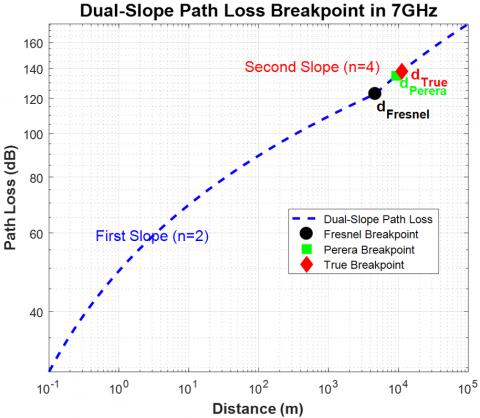
In Figure 3, when using a frequency of 7 GHz the breakpoint distance is located at 7 km for Fresnel, reaches 10 km for Perera, and is slightly more in True. However, Figure 4 shows the breakpoint at 10 GHz.
Figure 3. Fresnel, Perera, and True breakpoints in 7 GHz using dual slope path loss
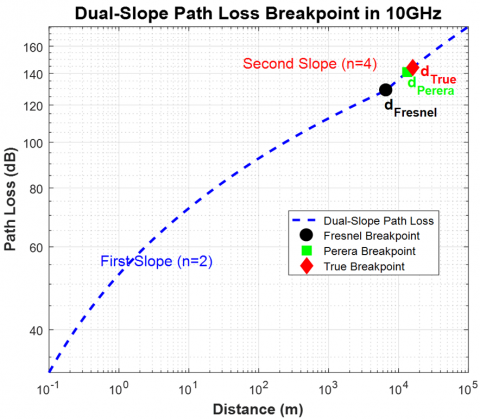
Figure 4. Fresnel, Perera, and True breakpoints in 10GHz using dual slope path loss
At 10 GHz, the Fresnel breakpoint is achieved at 8 km, while it is obtained at approximately 11 km and 12 km for Perera and True, respectively, clearly indicating to wireless link designers and planners that wavelength influences the breakpoint distance.
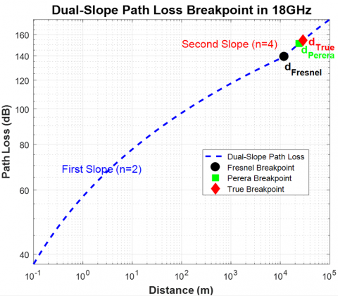
Moreover, Figure 5 presents the simulation using a frequency of 18 GHz, which could be used in mobile backhaul solutions. The results show a gradual increase in breakpoints, as illustrated in Figure 5.
At 18 GHz, the models exhibited remarkable growth, surpassing 10 km at the Fresnel breakpoint and reaching 15 km at Perera, while showing a slight increase at the True breakpoint. The results provide insight into the impact of frequency on breakpoint distance.
Figure 5. Fresnel, Perera, and True breakpoints in 18GHz using dual slope path loss
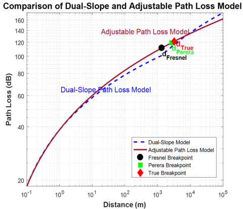
In contrast, the adjustable model demonstrates a gradual increase in the exponent, leading to a smoother and more realistic transition between propagation regions. This improvement is particularly evident in the transition region between the Fresnel, Perera, and True breakpoints, where the adaptive exponent reduces sudden jumps in signal attenuation. Figure 6 illustrates this concept, clearly distinguishing between them.
Figure 6. A comparison between dual slope and adjustable path loss models
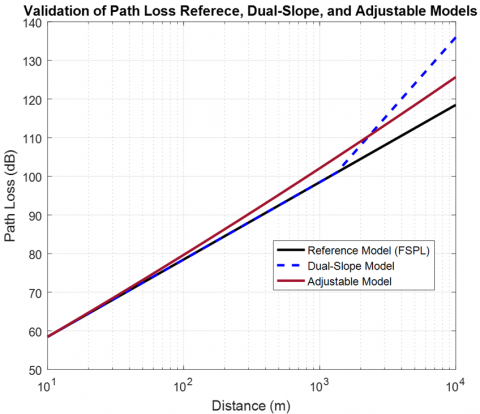
Nevertheless, the validation results in Figure 6 confirm that the Adjustable Dual-Slope Path Loss Model outperforms the traditional Dual-Slope Model in terms of stability and accuracy. The proposed model achieves remarkable consistency in RMSE as well, demonstrating its ability to provide more realistic path loss predictions with its steady behavior. However, a slight shift appears when reaching 1 km and beyond. While the Dual-Slope Model shows ideal validation up to 1 km, it then begins to exhibit notable severity beyond that, unless it reaches 135 dB path loss at 10 km. Figure 7 further illustrates that the adjustable model maintains significantly stable performance across distance values, proving its effectiveness in wireless propagation modeling.
Figure 7. Validation between dual slop and adjustable with FSPL reference
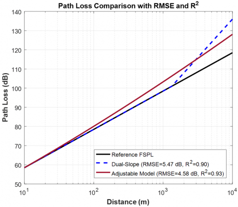
Consequently, RMSE was performed to verify the study and compare the dual-slope and adjustable models using FSPL as a reference. The validation provides significant results by equalizing the two models over short distances of up to 100 meters, while giving an advantage to the dual-slope model as the distance extends to 1 km. Beyond that, the adjustable model performs better due to the dual-slope model's significant decline over longer distances. In summary, the validation illustrated in Figure 8 employs R-squared (R²) and root mean squared error (RMSE) metrics to discover accurately the model’s calculations.
Figure 8. RMSE and R² calculation between dual slop and adjustable with FSPL reference
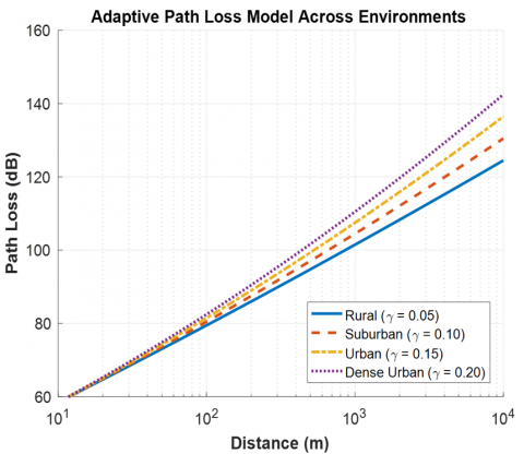
The adjustable model achieved an RMSE of 4.58 dB and R² = 0.938, compared to 5.47 dB and R² = 0.901 for the dual-slope model. This demonstrates a 16.2% reduction in error and a significantly improved fit to the reference FSPL model, validating the proposed model’s predictive strength. Whereas for more comparative analysis, the proposed model adapts to propagation environments by adjusting the exponent via a tuning parameter $\gamma$. As shown in Figure 9, environments with higher $\gamma$, such as dense urban areas, yield steeper path loss curves, while rural environments with lower $\gamma$ experience minimal attenuation over long distances. This adaptable structure allows the model to represent a variety of real-world deployment scenarios without the need for separate modelling equations.
It's worth noting that one limitation of this work is the absence of direct field measurement validation. However, the simulation data was generated using standardized propagation formulas and environments based on 3GPP TR 38.901. Nevertheless, the door remains open to extending the model to real-world datasets that would enhance robustness and assess practicality in dynamic environments.
Figure 9. Comparative analysis in different environments
This work proposes an improved dual-slope path loss model with an adjustable path loss exponent that seamlessly transitions between different propagation settings, particularly above 1 km, where the dual-slope model is severely prone to attenuation. The proposed technique computes path loss in a stepwise manner across Fresnel, Perera, and True breakpoints, resulting in steady and higher accuracy in urban and suburban propagation settings. The results indicate that frequency plays a crucial role, with higher frequencies experiencing greater path loss over distance. This underscores the importance of careful frequency selection. However, while the dual-slope model can be effective at shorter distances not exceeding a few kilometers, the adjustable model provides a more disciplined behavior by dynamically altering the exponent as a function of distance. This eliminates the harsh discontinuities found in typical dual-slope models, especially over kilometer-scale distances. Despite the use of an adjustable path loss exponent enhances accuracy by allowing for a seamless transition in attenuation behaviour. However, it introduces new model parameters, including the tuning factor, which may raise the challenge. But in fact, this difficulty is manageable and does not require large adaptations to existing wireless networks. The adaptability feature could be predefined for various environments (urban, rural, suburban), or dynamically adjusted using simple threshold logic or automated tuning based on terrain classification. Future studies will integrate intelligent reflection with breakpoint placements.
The author wishes to thank Sohar University in Oman for providing the resources and academic environment that facilitated the successful completion of this research.
[1] Wang, G., Chen, H., Li, Y., Jin, M. (2012). On received-signal-strength based localization with unknown transmit power and path loss exponent. IEEE Wireless Communications Letters, 1(5): 536-539. https://doi.org/10.1109/WCL.2012.072012.120428
[2] Ergen, S.C., Tetikol, H.S., Kontik, M., Sevlian, R., Rajagopal, R., Varaiya, P. (2013). RSSI-fingerprinting-based mobile phone localization with route constraints. IEEE Transactions on Vehicular Technology, 63(1): 423-428. https://doi.org/10.1109/TVT.2013.2274646
[3] Salman, N., Ghogho, M., Kemp, A.H. (2011). On the joint estimation of the RSS-based location and path-loss exponent. IEEE Wireless Communications Letters, 1(1): 34-37. https://doi.org/10.1109/WCL.2012.121411.110059
[4] Basheer, M.R., Jagannathan, S. (2013). Localization and tracking of objects using cross-correlation of shadow fading noise. IEEE Transactions on Mobile Computing, 13(10): 2293-2305. https://doi.org/10.1109/TMC.2013.34
[5] Elmutasim, I. (2023). A brief review of massive MIMO technology for the next generation. The International Arab Journal of Information Technology, 20(2): 262-269.
[6] El-Sallabi, H. (2011). Terrain partial obstruction LOS path loss model for rural environments. IEEE Antennas and Wireless Propagation Letters, 10: 151-154. https://doi.org/10.1109/LAWP.2011.2108254
[7] He, R., Zhong, Z., Ai, B., Ding, J., Guan, K. (2012). Analysis of the relation between Fresnel zone and path loss exponent based on two-ray model. IEEE Antennas and Wireless Propagation Letters, 11: 208-211. https://doi.org/10.1109/LAWP.2012.2187270
[8] Xia, H., Bertoni, H.L., Maciel, L.R., Lindsay-Stewart, A., Rowe, R. (2002). Radio propagation characteristics for line-of-sight microcellular and personal communications. IEEE Transactions on Antennas and Propagation, 41(10): 1439-1447. https://doi.org/10.1109/8.247785
[9] Oda, Y., Tsunekawa, K., Hata, M. (2000). Advanced LOS path-loss model in microcellular mobile communications. IEEE Transactions on Vehicular Technology, 49(6): 2121-2125. https://doi.org/10.1109/25.901884
[10] Milstein, L.B., Schilling, D.L., Pickholtz, R.L., Erceg, V., et al. (2002). On the feasibility of a CDMA overlay for personal communications networks. IEEE Journal on Selected Areas in Communications, 10(4): 655-668. https://doi.org/10.1109/49.136061
[11] Hernandez-Valdez, G., Cruz-Perez, F.A., Lara-Rodriguez, D. (2008). Sensitivity of the system performance to the propagation parameters in LOS microcellular environments. IEEE Transactions on Vehicular Technology, 57(6): 3488-3509. https://doi.org/10.1109/TVT.2008.919608
[12] Feuerstein, M.J., Blackard, K.L., Rappaport, T.S., Seidel, S.Y., Xia, H.H. (1994). Path loss, delay spread, and outage models as functions of antenna height for microcellular system design. IEEE Transactions on Vehicular Technology, 43(3): 487-498. https://doi.org/10.1109/25.312809
[13] Elmutasim, I.E., Mohd, I.I. (2020). Radio propagation in evaporation duct using SHF range. Publisher International Journal of Advanced Science and Technology IJAST Journal: Science and Engineering Research Support Society, SERSC Australia.
[14] Perera, S.C.M., Williamson, A.G., Rowe, G.B. (1999). Prediction of breakpoint distance in microcellular environments. Electronics Letters, 35(14): 1135-1136. https://doi.org/10.1049/el:19990834
[15] Galvan-Tejada, G.M., Aguilar-Torrentera, J. (2019). Analysis of propagation for wireless sensor networks in outdoors. Progress in Electromagnetics Research B, 83: 153-175. https://doi.org/10.2528/PIERB18100801
[16] Politi, R.R., Tanyel, S. (2025). Minimizing delay at closely spaced signalized intersections through green time ratio optimization: A hybrid approach with k-means clustering and genetic algorithms. IEEE Access, 13: 43981-43999. https://doi.org/10.1109/ACCESS.2025.3549970
[17] Jiang, T., Zhang, J., Tang, P., Tian, L., et al. (2021). 3GPP standardized 5G channel model for IIoT scenarios: A survey. IEEE Internet of Things Journal, 8(11): 8799-8815. https://doi.org/10.1109/JIOT.2020.3048992
[18] Safjan, K., D'Amico, V., Bultmann, D., Martin-Sacristan, D., Saadani, A., Schoneich, H. (2011). Assessing 3GPP LTE-advanced as IMT-advanced technology: The WINNER+ evaluation group approach. IEEE Communications Magazine, 49(2): 92-100. https://doi.org/10.1109/MCOM.2011.5706316
[19] Riviello, D.G., Di Stasio, F., Tuninato, R. (2022). Performance analysis of multi-user MIMO schemes under realistic 3GPP 3-D channel model for 5G mmWave cellular networks. Electronics, 11(3): 330. https://doi.org/10.3390/electronics11030330
[20] Hassija, V., Chamola, V., Mahapatra, A., Singal, A., et al. (2024). Interpreting black-box models: A review on explainable artificial intelligence. Cognitive Computation, 16(1): 45-74. https://doi.org/10.1007/s12559-023-10179-8
[21] Elmezughi, M.K., Salih, O., Afullo, T.J., Duffy, K.J. (2022). Comparative analysis of major machine-learning-based path loss models for enclosed indoor channels. Sensors, 22(13): 4967. https://doi.org/10.3390/s22134967
[22] Fernández, H., Rubio, L., Rodrigo Peñarrocha, V.M., Reig, J. (2024). Dual-slope path loss model for integrating vehicular sensing applications in urban and suburban environments. Sensors, 24(13): 4334. https://doi.org/10.3390/s24134334
[23] Mi, Y., Zhang, X., Liu, X., Wei, J. (2024). Measurement-based improved two-ray model for maritime scenarios. In 2024 6th International Conference on Communications, Information System and Computer Engineering (CISCE), Guangzhou, China, pp. 973-977. https://doi.org/10.1109/CISCE62493.2024.10653322
[24] Elmutasim, I.E., Mohamed, I.I., Bilal, K.H. (2023). Seawater salinity modelling based on electromagnetic wave characterization. International Journal of Electrical and Computer Engineering, 13(4): 4112-4118. https://doi.org/10.11591/ijece.v13i4.pp4112-4118
[25] Sun, Z., Liu, T., Wang, L. (2020). Analysis of DME signal strength in approach direction under two-ray model. In 2020 IEEE 2nd International Conference on Civil Aviation Safety and Information Technology (ICCASIT), Weihai, China, pp. 105-109. https://doi.org/10.1109/ICCASIT50869.2020.9368606
[26] El-Sallabi, H., Qaraqe, K. (2015). Correction terms of ground and water reflection surfaces for Perera’s breakpoint distance model. IEEE Antennas and Wireless Propagation Letters, 15, 786-789. https://doi.org/10.1109/LAWP.2015.2474698
[27] Kustysheva, I. (2017). Consideration of environmental factors in planning and development of urban areas. IOP Conference Series: Materials Science and Engineering, 262(1): 012166. https://doi.org/10.1088/1757-899X/262/1/012166