Saleem A. Ali*![]() | Theodore V. Hromadka
| Theodore V. Hromadka
© 2023 IIETA. This article is published by IIETA and is licensed under the CC BY 4.0 license (http://creativecommons.org/licenses/by/4.0/).
OPEN ACCESS
CVBEM is a numerical method of solving boundary value problems that satisfy Laplace's Equation in two dimensions. Three key parameters that impact the computational error and functionality of CVBEM are the basis function, the positions of the modeling nodes, and the coefficient determination methodology. To demonstrate the importance of these parameters, a case study of 2D ideal fluid flow into a 90-degree bend and over a semicircular hump was conducted comparing models using original CVBEM, complex log, complex pole, and digamma function variants basis functions, using two different NPAs, NPA1 and NPA2, and using collocation and least squares methods to determine coefficients. Results indicate that the combination of the original CVBEM basis function, NPA2, and least squares results in an approximation with the least computational error. Moreover, least squares appear to enable stability in both NPAs regarding reduction of computational error due to taking advantage of all boundary data and more stable condition number growth. By exploring the interaction of the three main CVBEM parameters, this paper clarifies the unique impact they have on the modelling process and explicitly identifies a fourth parameter, collocation point placement, as being impactful on computational error.
complex variable boundary element method, harmonic function, numerical solutions, least squares, computational fluid dynamics
The traditional computational methods of finite element, finite difference, control volume and similar, boundary element, meshless methods among others, use the problem boundary to develop a modeling node placement pattern. The literature contains numerous examples of model nodes being placed on the problem boundary and then an interpolation scheme is applied to develop an approximation function defined along the problem boundary. Indeed, model nodes are typically placed before any modeling is undertaken. The methodology discussed in the current paper, CVBEM, uses modeling results to determine computational error along the problem boundary for subsequent use in model node positioning. Algorithms have been developed to accomplish this search and adjustment task called Nodal Positioning Algorithms or NPA [1-3]. Thus, the model node distribution is developed as part of the presented modeling procedure. Use of nodes exterior of the problem domain are commonplace, however, because of the singularities typically involved with many types of basis functions, nodes are usually excluded from the problem interior. The final node distribution developed by application of the NPA (such as presented below) is therefore dependent not only upon the type of basis functions used in the approximation but the problem definition itself. Numerous tests of the presented computational procedure show that final node positions seldom occur on the problem boundary, but instead arise in the problem domain exterior such as seen in the example problem.
Use of the described modeling procedure has been highly successful in achieving computational error reduction in comparison to other computational methods such as domain methods and the like. In this paper, we use MATLAB software on a laptop as the computational engine. The presented methodology leverages application of a defined computational error to formulate model node spatial patterns from which a plot of computational error versus model number of nodes is developed as a modeling outcome.
1.1 The approximation function
The approximation function used is the linear sum of complex basis functions multiplied term-wise by complex coefficients. Complex coefficients are determined by equating the approximation with known values of the problem solution in a collocation process. Initially, the collocation process is part of an iterative process where approximation coefficients are determined in their entirety as a sequence of values for both the real and imaginary parts of each coefficient. Assuming that the domain of interest is a simply connected domain $\Omega \subset \mathbb{R}^2$ where Laplace’s equation holds, and $\Omega$ is an open set, the CVBEM approximation function is of the form:
$\widehat{\omega}(z)=\sum_{j=1}^n c_j g_j(z)$ (1)
where $c_j \subset \mathbb{C}$ is a complex coefficient, gi(z) is a complex variable function that is analytic within $\Omega$ and harmonic, and $n$ is the number of basis functions, or nodes, used in the approximation function [4, 5]. In contrast with real variable methods that utilize real coefficients, the complex coefficients consist of a real and imaginary part. Thus, for each basis function there are two degrees of freedom (DOF). In other words, for $n$ nodes, there are 2$n$ DOF that are determined by 2$n$ collocation points through collocation. The additional degrees of freedom could account for differences in computational error when comparing CVBEM to real variable methods.
$\frac{\partial u}{\partial x}=\frac{\partial v}{\partial y}$ (2)
$\frac{\partial u}{\partial y}=-\frac{\partial v}{\partial x}$ (3)
Because the approximation is comprised of harmonic functions, its real and imaginary parts are related through the Cauchy-Riemann Eqs. (2) and (3), and the potential lines and streamlines are orthogonal in the resulting flow net plot. Thus, when only the real or imaginary part can be modelled due to the available data, the other part can be easily determined using the Cauchy-Riemann equations [6, 7].
In summary, the three key parameters of the CVBEM methodology are the used basis functions, of which there is a diverse selection, the position of nodes, and the methodology to determine the approximation function coefficients. Numerous studies have explored the impact of these three parameters on the resultant models, especially in computational error.
1.2 Basis functions
The basis function to be used is an important consideration of the CVBEM modelling process. To ensure that linear combinations of basis functions are harmonic and satisfy the Laplace equation over the problem domain, the selected basis functions are analytic. The underpinnings of this process can be found in publications prepared by Walsh, which predates the advent of the digital computer, where he proves several theorems regarding the approximation of complex analytic functions bounded by Jordan arcs [8, 9].
The family of basis functions that can be used for CVBEM modelling is any harmonic function that is analytic in the problem domain of interest. Previous research has explored the application of the following basis functions in CVBEM modelling and has illustrated that the main difference is how fast the approximation function converges [10].
Depending on the selected basis function, special considerations may need to be taken such as rotating the branch cuts of the complex natural logarithm so that each branch lies in the exterior of the problem domain. Consequently, the resulting approximation function will be analytic within the problem domain [10].
1.3 Location of nodes
It has been illustrated that the computational error of CVBEM and other methods tends to decrease as the number of nodes increase, but a long standing issue has been how to choose the location of the nodes and collocation points [3, 11, 12]. In this regard, there are two main approaches: one is when the node locations are determined. Various node distributions where node locations are determined have been assessed, such as nodes uniformly spaced on a circle, nodes located a constant distance away from the problem boundary, and nodes on an evenly spaced grid around the problem domain [11]. Because the node locations are predetermined, there is high computational efficiency, but the computational accuracy of the models is unreliable. Thus, treating the node locations as another set of degrees of freedom is an alternative method that has been illustrated to reduce computational error [1-3, 11, 12]. The most recent algorithms developed for CVBEM but is also applicable to other methods like the Method of Fundamental Solutions is called the Node Positioning Algorithm (NPA1) and its refinement procedure (NPA2) [3].
1.3.1 NPA1 vs NPA2
NPA1 works as described in the following steps:
1. Generate two sets of points: Candidate nodes and candidate collocation points. Candidate nodes are located on the exterior of the problem domain, and candidate collocation points are located on the domain boundary.
2. Select two initial collocation points to be used for collocation. Two collocation points are necessary because complex coefficients have two degrees of freedom, a real and imaginary part. From this point the NPA starts.
3. For each candidate node, create a model and evaluate its error. Select the model that results in the least maximum error on the boundary.
4. Evaluate the error of the selected model and select the next two collocation points to be the two greatest maxima of the error function.
5. Repeat steps 3 and 4 until the desired number of nodes is achieved.
NPA1 provides a methodology to select nodes with the intention of reducing the computational error of the model. Experimental results have illustrated its efficacy, but there it possesses a significant drawback. That is, NPA1, when selecting a new node, operates under the assumption that the selected nodes are correct. In other words, it does not consider the possibility that computational error can be reduced by adjusting the position of the previously selected nodes. Consequently, a refinement procedure was developed that specifically addresses this problem and named it NPA2. The following steps describes NPA2:
In contrast with NPA1, NPA2 adjust every node’s position instead of solely the new node being added to the model, which results in lower computational error at the expense of time due to its greater complexity [3]. In summary, both NPA’s provide a better methodology for selecting nodes instead of using predetermined node locations and has been illustrated to reduce computational error in problems CVBEM has been historically used to solve, such as modelling the transportation of ground water contamination [1, 13].
1.4 Coefficient determination method
Most recently, CVBEM research has looked at the method of determining coefficients of the approximation function as another avenue of customization of the CVBEM modelling process [14]. For nearly 40 years, collocation has been the foremost method for coefficient determination. However, a recent advancement was the development of a least squares methodology. The main difference between the two methods is how the collocation points are used. As described in Section 1.1, collocation prescribes 2 collocation points for each node to determine the coefficients. Thus, if there were N total candidate collocation points and a n node model was being made, N-2n collocation point would have no effect on the model. The advantage of collocation is that the approximation function will satisfy the boundary conditions at the used collocation points with zero error. Conversely, least squares takes advantage of all available boundary data to compute the coefficients of the approximation. However, instead of exactly satisfying a subset of collocation points, it instead minimizes the sum of the squares of the error between the approximation and all the collocation points. Despite not exactly fitting any of the boundary conditions, using least squares has resulted in comparable computational error to collocation.
1.5 Computational error analysis
In this work, we define computational error function as magnitude of the difference between the CVBEM approximation function and the known boundary function, $f(z)$:
$E=\|f(z)-\widehat{\omega}(z)\|$ (4)
Because the CVBEM approximation function is a linear combination of functions analytic in the problem domain, thus it itself is also analytic within the problem domain. It follows that the real and imaginary parts of the problem domain are related through the Cauchy-Riemann equations, so the real and imaginary parts are consequently harmonic. As a result, because the target function and CVBEM approximation functions are both harmonic, their difference, which is the error function, is also harmonic. This property is pivotal in the error analysis of CVBEM approximation functions because the maximum and minimum principle of harmonic functions, which states that the maximum and minimum values of a harmonic function are located on the boundary of its domain. Therefore, because the error function is harmonic, it is known that the point of maximum error is located on the boundary of $\Omega$. When the error of CVBEM models is plotted for comparison, the maximum error is plotted against the number of nodes in the model, which is equivalent to the number of terms in the CVBEM approximation function. While the computational error of CVBEM models has always been assessed in the literature in regard to its magnitude, this paper seeks to reveal more about intricacies of the error’s behavior throughout the modeling process.
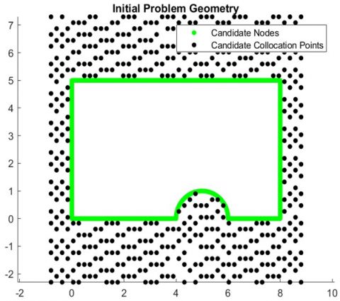
A case study is used to demonstrate the results of the CVBEM modeling procedure. It is ideal fluid flow into a 90 degree bend and over a semicircular hump. This problem was selected because it contains three stagnation points located at the 90 degree bend and at the left and right ends of the hump. Due to the extreme curvature of solutions at stagnation points, they are particularly difficult to model. Similarly, the north pole of the semicircular hump exhibits extreme curvature, which make it a difficult are to model. This complexity requires the use of more nodes to be effective in reducing error, which will make it easier to observe trends in error reductions. The exact definition of this example problem is found in Table 1 and the initial problem geometry is depicted in Figure 1.
Table 1. Problem definition
|
Problem Domain |
$\Omega=\{0 \leq x \leq 8,0 \leq y \leq 5 \, \text{ and } \,(x-5)^2+y^2 \geq 1\}$ |
|
Governing PDE |
$\nabla^2 \Psi=0$ |
|
Boundary Conditions |
$\Psi(x, y)=\Re\left[z^2+z+\frac{10}{z-5}\right]$ |
|
Candidate Nodes |
500 |
|
Candidate Collocation Points |
1000 |
|
Selected Nodes |
40 |
|
Selected Collocation Points |
80 |
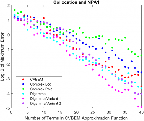
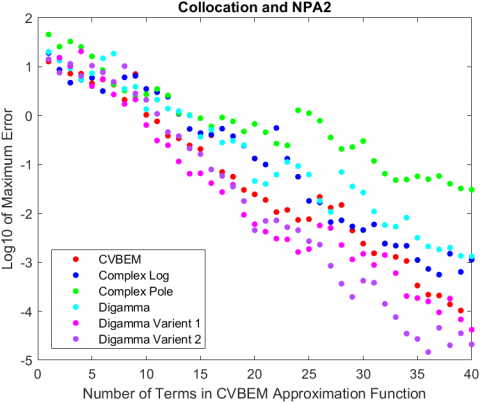
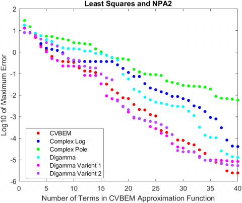
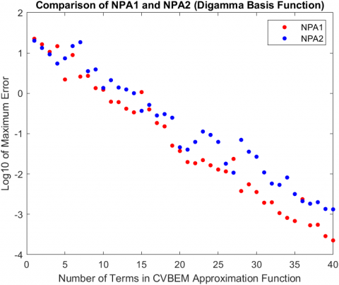
The main results of this case study are presented in Figure 2, where the log10 of the maximum error for each of the models is plotted. For collocation and NPA1, the model that resulted in the lowest maximum computational error used digamma variant 1 as the basis function and achieved a maximum error of 1.190995×10⁻⁵. The digamma variant 2 basis function achieved 2.100197×10⁻⁵ as the lowest maximum computational error for collocation with NPA2. Digamma variant 1 also had the lowest maximum computational error for least squares with NPA1, which was 2.110717×10⁻⁵. Finally, the model that resulted in overall lowest maximum error used least squares, NPA2, and the CVBEM basis function. Its error was 2.465528×10⁻⁶.
Figure 1. Initial distribution of candidate nodes and collocation points for every model
Clearly, different combinations of basis functions, NPAs, and methods to determine coefficients produce different error, and the results replicate previous findings. Figure 2 illustrates that the different basis functions affected the rate at which the numerical solution converges, with digamma variant 1, digamma variant 2 and the CVBEM basis function converging the fastest in their respective modelling scenario.
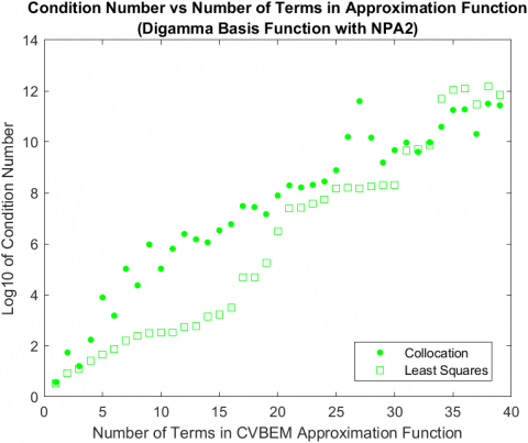
Results regarding the NPAs support NPA2’s greater relative error reduction capability compared to NPA2, with two exceptions: using collocation, the digamma and digamma variant 1 basis functions had more computational error when NPA2 was applied compared to NPA1 (see Figure 3). In both cases, NPA2 starts off with less error, but eventually its error overtakes the error of NPA1. This highlights the potential for NPA2 to select a path of nodes that results in greater error in NPA1 despite the refinement procedure that NPA2 implements. A potential explanation is the order of the nodes that the refinement procedure is applied to. In other words, in the same vein that NPA1 was flawed, NPA2 exhibits the same flaw when it starts its refinement procedure from the first selected node, which can lead to different model from NPA1 but not necessarily one with less computational error. This is further supported by Figure 4, where there is a large spike at the 27th term for the condition number of collocation that coincides with the spike in maximum computational error observed in Figure 2. In essences, the node that ends up being selected causes the condition number to increase greatly when compared to the expected increase the come with a growing matrix, which ultimately results in more computational error. One potential mitigation for this issue is to increase the number of candidate nodes, which will give both NPAs more nodes to choose from, which could strengthen the error reduction due to refinement in NPA2. This can be done by increasing the density of candidate nodes in the candidate node space or by expanding the candidate node space and maintaining the density.
When least squares was considered alongside collocation, in addition to ultimately resulting in the model with the least computational error, the error plots also demonstrated a distinct stability in error reduction.
That is, for both NPA1 and NPA2, the error plots for least squares demonstrate a monotonic reduction in computational error, whereas the collocation models have occasional increases in computational error as seen in Figures 3A and 3B. This can be attributed to differences in how collocation and least squares handle the boundary data. For collocation, because the information the approximation has concerning the boundary of the problem is limited to the collocation points it utilized, what happens is at the start of the algorithm is selected collocation points could be clustered withing a certain region of the problem boundary, so the model approximates that part of the problem well. However, the regions with no collocation points are poorly approximated, which eventually causes the spike in error. The NPAs actually account for this by selecting new collocation points at the two highest maxima of the error function, which is why the error starts to decrease again. In contrast, because least squares utilizes all of the boundary data, as more nodes are added to the approximation, the error across the boundary decreases, not just around a few selected collocation points. This is reflected in the condition number for least squares, where it grows with relative stability and no spikes.
(A)
(B)
(C)
(D)
Figure 2. Log10 error for each of the created models plotted against the number of terms in the CVBEM approximation function
(A)
(B)
Figure 3. Error plots for the digamma and digamma variation 1 basis functions using collocation
Figure 4. Log10 of condition number plotted against the number of approximation terms
Improving the CVBEM process generally means reducing computational error. Investigations into new basis functions and NPA's are the primary avenue through which improvement has been sought. However, it has been illustrated that the selection method for collocation points and the coefficient determination method also have import effects on computational error. Thus, advancement can be focused in these four areas.
It has been well established by this paper and previous papers that different basis functions have different rates of convergence. A potential avenue of advancement is using multiple different basis functions within the same approximation. In other words, instead of each term in the approximation function being of the same basis function, the CVBEM algorithm selects the best node and basis function combination for each term. Through this, computational error can be reduced because the approximation could now be a better representation of the actual solution. For instance, the function that was being approximated in this case study was $z^2+z+\frac{10}{z-5}$, which consists of two complex monomials and a complex pole. Using both of those types of basis functions in an approximation would be a better representation of the actual problem and could lead to being able to accurately model the problem with less nodes.
Regarding the NPA and collocation point selection, this paper explained how spikes in error can occur due to poor node and collocation point selection. Currently, the NPA selects the two highest maxima of the error function as collocation points, which allows those same points to have essentially no error in the subsequent model. However, this can lead to sections of the problem boundary having no collocation points, which can cause a spike in error. A potential alternative collocation point selection method is to have the subsequent collocation points be furthest from the selected collocation points by average distance. This may enable the collocation method to use a more diverse portion of the problem boundary, which may reduce the spikes in error.
Finally, while least squares was previously illustrated as a viable coefficient determination method, and the distinctive characteristic of using all available boundary data was noted in a previous study, analysis of its effect on the behavior of the error and error reduction potential was not conducted. The observed stability of the error in least squares when compared to collocation is grounds to explore the impact of other coefficient determination methods. For instance, to address the increasing condition number as the number of nodes in the approximation increases, methods that utilize preconditioning could increase the rate of convergence through reduction of the condition number.
In addition to computational error reduction, another future investigation for CVBEM is shifting from 2D to 3D, which would allow more comprehensive models to be made. The biggest challenge here is the increase in the size of the domain, which would exacerbate the issue with collocation point selection. Consequently, least squares may prove to be better suited to 3D applications.
This work was supported by Captain Bryce D. Wilkins, whose knowledge of CVBEM assisted us in understanding the NPAs and the overall CVBEM methodology.
|
$c$ |
complex node coefficient |
|
$\mathbb{C}$ |
set of complex numbers |
|
CVBEM |
complex variable boundary element method |
|
$E$ |
computational error function |
|
$f$ |
boundary condition function |
|
$g$ |
approximation term/basis function |
|
$n$ |
number of nodes in approximation function |
|
NPA |
mode positioning algorithm |
|
$\mathbb{R}$ |
set of real numbers |
|
$\Re$ |
real part |
|
$z$ |
complex variable, $x+i y$ |
|
Greek symbols |
|
|
$\Omega$ |
simply connected domain |
|
$\psi$ |
digamma function |
|
$\widehat{\omega}$ |
CVBEM approximation function |
|
Subscripts |
|
|
$\alpha$ |
Clockwise rotation angle of digamma axis and natural log branch cut |
|
$j$ |
node index |
[1] Wilkins, B.D., Hromadka II, T.V., Nevils, W., Siegel, B., Yonzon, P. (2021). Using a node positioning algorithm to improve models of groundwater flow based on meshless methods. The Professional Geologist, 58(2): 54-61.
[2] Doyle, A., Nelson, A., Yuan, M., DeMoes, N.J., Wilkins, B.D., Grubaugh, K.E., Hromadka II, T.V. (2020). Advances in the greedy optimization algorithm for nodes and collocation points using the method of fundamental solutions. Engineering Analysis with Boundary Elements, 111: 148-153. https://doi.org/10.1016/j.enganabound.2019.10.018
[3] Wilkins, B.D., Hromadka II, T.V., McInvale, J. (2020) Comparison of two algorithms for location computational nodes in the Complex Variable Boundary Element Method (CVBEM). International Journal of Computational Methods and Experimental Measurements, 8(4): 289-315. https://doi.org/10.2495/CMEM-V8-N4-289-315
[4] Wilkins, B.D., Hromadka II, T.V. (2021). Foundations of the CVBEM. In Excel in Complex Variables with the Complex Variable Boundary Element Method. Southampton, UK: WIT Press, 137-201.
[5] DeMoes N.J., Bann G.T., Wilkins, B.D., Hromadka II, T.V., Boucher, R. (2019) 35 years of advancements with the complex variable element method. International Journal of Computational Methods and Experimental Measurements, 7(1): 1-13. https://doi.org/10.2495/CMEM-V7-N1-1-13
[6] Wilkins, B.D., Hromadka II, T.V. (2021). Using the digamma function for basis functions in mesh-free computational methods. Engineering Analysis with Boundary Elements, 131: 218-227. https://doi.org/10.1016/j.enganabound.2021.06.004
[7] Hromadka II, T.V., Guymon, G.L. (1984). A complex variable boundary element method: Development. International Journal for Numerical Methods in Engineering, 20: 25–37. https://doi.org/10.1002/nme.1620200104
[8] Walsh, J.L. (1929) On approximation by rational functions to an arbitrary function of a complex variable. Transactions of the American Mathematical Society, 31(3): 477-502. https://doi.org/10.2307/1989529
[9] Walsh J.L. (1935). Interpolation and approximation by rational functions in the complex domain. Providence, RI, USA: American Mathematical Society.
[10] Wilkins, B.D., Hromadka II, T.V., Johnson, A.N., Boucher, R., McInvale, H.D., Horton, S. (2018). Assessment of complex variable basis functions in the approximation of ideal fluid flow problems. International Journal of Computational Methods and Experimental Measurements, 7(1): 45-56. https://doi.org/10.2495/CMEM-V7-N1-45-56.
[11] Chen C.S., Karageorghis A., Li Y. (2015). On choosing the location of the sources in the MFS. Numerical Algorithms, 72: 107-130. https://doi.org/10.1007/s11075-015-0036-0
[12] Hromadka II, T.V., Zillmer, D. (2012) Boundary element modeling with variable nodal and collocation point locations. Advances in Engineering Software, 43(1): 96-103. https://doi.org/10.1016/j.advengsoft.2011.07.003
[13] Yen, C.C., Hromadka II, T.V., Lai, C. (1986). The complex variable boundary element method in groundwater contaminant transport. Proceedings: International Conference on Computational Mechanics (ICCM86 Tokyo), Springer-Verlag, XI-137-XI-142.
[14] Wilkins, B.D., Hromadka II, T.V. (2022). A least squares approach for determining the coefficients of the CVBEM approximation function. International Journal of Computational Methods and Experimental Measurements, 10(3): 237-259. https://doi.org/10.2495/CMEM-V10-N3-237-259