Aidel Sofiane![]() | Mourad Hamimid*
| Mourad Hamimid*![]()
© 2023 IIETA. This article is published by IIETA and is licensed under the CC BY 4.0 license (http://creativecommons.org/licenses/by/4.0/).
OPEN ACCESS
Iron losses are a major source of inefficiency in electrical devices, such as transformers and rotating machines. Accurately estimating iron losses is essential for optimizing the performance, energy efficiency, and cost-effectiveness of these devices. The swelling phenomenon is a significant factor that affects the accuracy of iron loss estimation. This phenomenon appears in the saturation region of the hysteresis loop under high-frequency regimes and can significantly affect the magnetic properties of the device. This paper presents a novel methodology for addressing the swelling phenomenon and improving the accuracy of iron loss estimation. The methodology is based on the Jiles-Atherton model, which is a well-established model for describing the hysteresis phenomenon in ferromagnetic materials. The methodology is improved by incorporating a novel formulation of the excess field based on magnetic viscosity. The Bertotti approach is used to account for the dynamic effects of the swelling phenomenon. The fmincon algorithm is used to identify the parameters of the Jiles-Atherton model in both quasi-static and dynamic regimes. This algorithm is a MATLAB®-based constrained optimization method that is used to find the set of parameters that minimizes the error between the simulated and measured hysteresis loops. The obtained results show that the proposed methodology is able to accurately estimate iron losses under both quasi-static and dynamic regimes.
hysteresis, swelling phenomenon, Jiles-Atherton model, Bertotti approach, magnetic viscosity
Designing electromagnetic devices optimally requires selecting materials with improved magnetic and electrical properties. The precise evaluation of iron losses in magnetic materials is a significant challenge in magneto-dynamics. The advancement of power electronics and control systems, such as electrical machines, has evolved to operate at higher frequencies. This development has enabled a wider range of applications and the ability to reduce the size of actuators while maintaining the same power output. However, higher frequencies also result in increased iron losses in electric machines, making it crucial to accurately predict and model these losses for efficient design and operation. These losses can represent through a phenomenon where the hysteresis loop of a magnetic material expands or increases in size when the frequency of the magnetic field applied to the material is increased. This swelling hysteresis effect has implications for iron losses in electric machines, as it influences components of iron losses, such as eddy current losses and excess losses [1]. Various models have been proposed in the literature [2, 3] to address this issue. The incorporation of the dynamic Jiles-Atherton model into a numerical simulation of iron losses evaluation is an effective tool for modeling and predicting the losses of electrical steel laminations, as confirmed by several works [4, 5]. Usually, the dynamic models based on the Jiles-Atherton one, have been built on Bertotti’s theory [6-9].
The central concept of this approach is based on the statistical approach of losses commonly referred to as the loss separation approach developed by Bertotti et al. [10]. Energy loss is divided into three components namely hysteresis (static) loss or magnetic energy loss is usually separated into a frequency-independent hysteresis contribution Whys, and a frequency-dependent dynamic contribution Wdyn such as classical eddy current loss Wcla, and excess loss Wexc. The total energy loss is represented as the sum of these components, and this framework is widely used to calculate the iron losses in non-oriented (No) and grain (Go) materials [7, 11]. An alternative approach based on magnetic viscosity provides the ability to represent the characteristic of the hysteresis phenomenon and to control the shape of the dynamic hysteresis loop, through this approach, modeling the process of incorporating dynamic effects into the static hysteresis model to accurately represent the behavior of soft magnetic materials [12]. This is achieved by introducing a viscous-type equation that describes the time delay of induction B behind the applied field H. The dynamic loop of the magnetization process can be expanded, allowing for a more accurate representation of the material's response to changing magnetic fields.
Based on this approach, several studies have been conducted using this approach to incorporate the Jiles-Atherton model into a dynamic regime using magnetic viscosity [13, 14]. Although the results obtained from these attempts were consistent with measurements, they encountered a significant challenge at high-frequency levels when a deformation or so-called swelling appears in the saturation region of the hysteresis loop. This requires prior knowledge of the magnetic flux density level at the site of swelling, which presents a drawback in the application of these approaches.
To address this limitation, this paper proposes an improved excess field expression that includes functions of magnetic flux density B for the two constant parameters αexc and gexc. The parameter αexc offers the possibility to control the shape of hysteresis loops which has been modified as a function to find the variation of magnetic field Hdyn. These functions have four parameters with the five parameters of JA. A MATLAB®-based constrained optimization algorithm called fmincon is used to identify the parameters of the JA model in both quasi-static and the four parameters in dynamic regimes by calculation error quadratic between calculated and measurement. The fmincon algorithm is capable of handling non-linear functions, constraints, and decision variable bounds. The proposed methodology is validated by calculating dynamic hysteresis loops and comparing the results to measurements. The proposed approach was validated by comparing its results with non-oriented Fe-Si (M400-50A) measurements in the frequency range of 10 to 1000 Hz [15].
2.1 Original JA hysteresis model
In the original Jiles-Atherton hysteresis model (JA) [16], the total magnetization (M) is divided into two parts: reversible magnetization (Mrev) and irreversible magnetization (Mirr). The reversible magnetization accounts for the translation and reversible rotation of domain walls during the magnetization process. It represents the elastic response of the material to the applied magnetic field. On the other hand, irreversible magnetization corresponds to the displacement of domain walls overcoming pinning forces. The relationships between the two components and anhysteretic magnetization (Man) are established based on the physical principles that govern the magnetization process.
The primary equations within this model are as follows:
$\frac{d M_{i r r}}{d H_e}=\frac{M_{a n}-M_{i r r}}{k \delta \alpha\left(M_{a n}-M_{i r r}\right)}$ (1)
$M_{e r v}=c\left(M_{a n}-M_{i r r}\right)$ (2)
$H_e=H+\alpha M_{i r r}$ (3)
$M_{a n}=M_s\left(\operatorname{coth}\left(\frac{H_e}{a}\right)-\frac{a}{H_e}\right)$ (4)
Finally, the total differential susceptibility, dM/dH, was determined in the customary form.
$\frac{d M}{d H}=(1-c) \frac{\left(M_{a n}-M_{i r r}\right)}{k \delta-\alpha\left(M_{a n}-M_{i r r}\right)}+c \frac{d M_{a n}}{d H_e}$ (5)
where, He, Man, and Ms are, respectively, the effective field, the anhysteretic magnetization, and the saturation, magnetization. a, α, c, and k and are the model parameters where a represent quantified domain wall density. α is the parameter of inter-domain coupling. c is the coefficient magnetization reversibility and k represent quantified energy to break the pinning site in ferromagnetic materials, these parameters have to be determined from measured hysteresis characteristics, δ is a directional parameter takes the sign of dH/dt.
2.2 Inverse JA hysteresis model
The Jiles-Atherton hysteresis model initially uses the applied magnetic field (H) as the independent variable. In the inverse Jiles-Atherton model, the magnetization (M) is determined based on the magnetic flux density (B). This is achieved by integrating a differential equation with respect to the rate of change of magnetization with respect to magnetic flux density (dM/dB). The inverse JA hysteresis model is given as [17]:
$\frac{d M}{d B}=\frac{\xi}{\mu_0(k \delta+(1-\alpha) \xi)}$ (6)
$\xi=\delta k c \frac{d M_{a n}}{d H_e}+\left(M_{a n}-M\right)$ (7)
$\frac{d M_{a n}}{d H_e}=\frac{M_s}{a}\left(1-\operatorname{coth}\left(\frac{H_e}{a}\right)^2-\left(\frac{a}{H_e}\right)^2\right)$ (8)
Using a JA model for modeling magnetic hysteresis loops in a dynamic regime requires careful choice of a dynamic contribution approach. Previous research has introduced the concept of adding two opposing fields, introducing eddy currents, and expressing excess fields in the effective field using the concept of the separation of energy loss theory [7]. This approach provides a clear and systematic method for extending the JA model from a quasi-static to a dynamic regime, and has yielded acceptable results. The concept has been further enhanced by introducing a novel expression for excess losses based on magnetic viscosity and the JA model. This approach allows for the optimal shaping of the hysteresis loops by varying the exponent of the excess field expression [14].
In the study of Zirka et al. [12], researchers proposed an alternative approach based on magnetic viscosity. This approach has proven to accurately predict losses and control anomalous loop shapes by adjusting the exponent of the excess field expression along with some parts of the loop. This approach is a mathematical expression derived from Landau Gilbert’s equation in order to put the similarity between rotational magnetization and the time delay of induction B behind the applied field H [18]. From this has been derived the excesses field based on the magnetic viscosity equation.
For this, several attempts based on the magnetic viscosity approach have been proposed in the literatures [13, 14]. These studies yielded acceptable results, but they relied on prior knowledge of the magnetic flux induction level where swelling occurs.
Based on the separation of energy loss theory, the total field H(t) is decomposed also into three components, hysteresis field Hhys(t), classical eddy-current field Hedd(t), and excess field Hexc(t). The total field can be represented as follows:
$H(t)=H_{h y s}(t)+H_{e d d}(t)+H_{e x c}(t)$ (9)
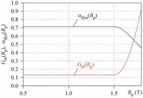
Here Hhys(t) is the magnetic field calculated by using the inverse Jiles-Atherton model (Eq. (6) to Eq. (8)). As well as Eq. (10) below gives the excess field expression, where αexc(Bp) is given as a function that represents a variable in the equation that describes the behavior of losses in a magnetic material [19]. Its physical meaning account for random spatial variations in domain size and domain wall number [20]. This function affects the losses at different levels of flux density (Bp). Incorporating αexc(Bp) provides more precise predictions of losses, especially at higher frequencies. The Figure 1 below illustrates the evolution of the parameters Gm(Bp) and αdyn(Bp) in correlation with peak induction values.
Figure 1. Peak-induction dependencies in GO Steel: Gm(Bp) and αdyn(Bp) [19]
$H_{e x c}(t)=\delta g_{e x c}(B)\left|\frac{d B}{d t}\right|^{\alpha_{e x c\,\,\,}\left(B_p\right)}$ (10)
where, gexc(B) is dynamic magnetic resistivity, that controls the shape of the dynamic hysteresis loop, and its simplest form is given as a polynomial by [19, 21]:
$g_{e x c}=C_1\left(1+C_2 B^2\right)$ (11)
The shape of the dynamic hysteresis loop is influenced by two constants, C1 and C2. These constants play an important role in determining the waist and area of the loop, and as a result, they have a significant impact on the shape of the loop in the saturation region. By adjusting the values of C1 and C2, it is possible to control the shape of the dynamic hysteresis loop.
The classical eddy-current field is given as [22]:
$H_{e d d}=k_{e d d} \frac{d B(t)}{d t}$ (12)
kedd is a coefficient related to the physical and geometrical parameters of the material and is given by [23]:
$k_{e d d}=\frac{\sigma d^2}{2 \beta}$ (13)
where, σ is the conductivity of the material, d and β are parameters related to the geometry of the material. In the case of a sheet, d corresponds to the thickness of the sheet, and β is a form factor.
Another approach gives αexc as a function of the magnetic flux density B(t) instead of a constant or as a function of the pic induction (Bp) is proposed in this work. Eq. (14) shows the new form of αexc as a function of B(t).
$\alpha_{\text {exc }}(B(t))=1-C_3 \exp \left(-\delta C_4 B(t)\right)$ (14)
where, C3 and C4, are two constants that offer the possibility to control the swilling shape of hysteresis loops. δ is the same directional parameter. Eq. (14) is similar to Eq. (9) in the study of Reinert et al. [24]. This equation has proved the influence of premagnetization in ferromagnetic and ferromagnetic by new parameters as a function adapted to the influence of premagnetization, which adjusts the parameter of the Steinmetz equation. From a physical viewpoint, the variable αexc(B(t)) in Eq. (14) may be defined by the usage of the variation velocity normalized of the domain walls [25]. The main advantage of Eq. (14) does not need the preknowledge of magnetic flux density reversal of previous works [13, 14, 19]. They need to determine the level of the magnetic induction in the shape of the loop for modeling the swelling.
Introducing Eq. (14) and Eq. (12) in Eq. (9), the total magnetic field has the following form.
$\begin{gathered}H(t)=H_{h y s}(B)+k_{e d d} \frac{d B(t)}{d t}+ \delta g_{\text {exc }}(B)\left|\frac{d B}{d t}\right|^{\alpha_{\text {exc }}(B(t))}\end{gathered}$ (15)
This section is devoted to presenting the results of our proposal on hysteresis loops in both quasi-static and dynamic regimes. The main objective is to investigate and model hysteresis loops, which are commonly observed in the difference between measured and calculated. Through this proposal, the calculation of the iron losses in M400-50A materials in a dynamic regime. To achieve this, we employed different methods to model hysteresis loops and dynamic regimes.
4.1 Quasi-static regime
The proposed methodology for modeling the magnetic behavior of materials was validated using measurements from non-oriented (NO) magnetic sheets made of Fe-Si (M400-50A), as specified in the study of Baghel et al. [13].
These sheets have a thickness of 0.5 mm and a mass density of 7670 g/dm3.
Table 1. Quasi-static JA parameters
|
Parameter |
Value |
|
Ms (A/m) |
1.25×10⁶ |
|
a (A/m) |
57.14 |
|
k(A/m) |
55 |
|
c (-) |
0.081 |
|
α (-) |
1.15×10⁻⁴ |
The parameter values of the quasi-static (10 Hz) JA hysteresis model were determined using a MATLAB®-based constrained optimization algorithm called fmincon. Table 1 presents the obtained parameters. Figure 2 provides a comparison between the computed hysteresis loop and the measured one at 10 Hz.
The close agreement observed between the computed and measured hysteresis loops, as depicted in Figure 2, obtained under the quasi-static regime (10 Hz), not only provides strong support for the accuracy of the values presented in Table 1, but also highlights the effectiveness of the fmincon algorithm in accurately identifying the parameters of the Jiles-Atherton model.
Figure 2. Computed and measured hysteresis loop at 10 Hz
Figure 3 visually illustrates the progressive evolution of the fitness function over successive iterations. This function, which quantifies the discrepancies between measured and computed magnetic fields, demonstrates a discernible trend that reinforces the effectiveness of the optimization process. The continuous improvement observed in the fitness function affirms the algorithm's iterative convergence towards an optimal solution.
Figure 3. The evolution of the fitness function versus the number of iterations
4.2 Dynamic regime
In this regime, the five parameters derived in the quasi-static regime remain constant and unchanged, as indicated in Table 1. In the first approach, it is assumed that gexc(B) is constant and equal to kexc. With this assumption, Eq. (15) mentioned above can be expressed as follows:
$H(t)=H_{h y s}(B)+k_{e d d} \frac{d B(t)}{d t}+\delta k_{\text {exc }}\left|\frac{d B}{d t}\right|^{\alpha_{e x c\,\,\,}(B(t))}$ (16)
Four dynamic parameters characterize this equation; kedd, kexc, C3, and C4. The latter two parameters, C3 and C4, are associated with the parameter αexc(B(t)). The identification of these dynamic parameters was performed at an arbitrary frequency of 200 Hz, and their corresponding values are provided in Table 2.
Table 2. Dynamic parameters
|
Parameter |
Value |
|
kexc |
0.085 |
|
kedd |
0.030 |
|
C3 |
0.125 |
|
C4 |
1.520 |
Using Eq. (14) with the obtained parameters C3, and C4, the evolution of the parameter αexc is presented in Figure 4.
Figure 4 demonstrates how the parameter αexc changes as the magnetic flux induction B(t) varies, in both the ascending and descending branches of the hysteresis loop. As can be observed, the parameter ranges from −0.22 to 0.98.
The computed hysteresis loops are presented in Figure 5, compared to the measurements given in the study of Petrun and Steentjes [15] at different frequencies. As shown in the figure, Eq. (16) accurately provides accurate computed hysteresis loops at frequencies less than 400 Hz.
However, as the frequency exceeds 400 Hz, the computed hysteresis loops do not fit the measured ones, particularly in the saturation region where swelling occurs, as demonstrated in Figure 6.
Figure 4. Evolution of the parameter aexc
Figure 5. Computed and measured hysteresis loops Below 400 Hz frequencies
Figure 6. Discrepancy between computed and measured hysteresis loops beyond 400 Hz frequency
To enhance the precision of the computed hysteresis loops, the second approach introduced more refined modeling by considering both gexc(B) and αexc(B) as functions of B(t). The equation for gexc(B) is given by Eq. (11). The dynamic parameters, which are listed in Table 2, remained constant while the gexc coefficients were determined using an arbitrary frequency of 200 Hz. Table 3 presents the optimized values for C1and C2.
Table 3. gexc parameters
|
Parameter |
Value |
|
C1 |
0.085 |
|
C2 |
0.120 |
As shown in Figure 7, the parameter gexc exhibits a minimum value equivalent to C1=0.085 when the flux density (B) is zero, and a maximum value of 0.107 when the absolute value flux density is 1.5 T. The figure depicts the variation of gexc with B(t) using Eq. (15) and the obtained values of C1and C2.
Figure 7. Evolution of the parameter gexc
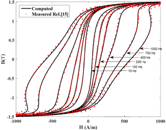
As seen in Figure 8, Eq. (15) provides close agreement between the computed hysteresis loops and the measured ones, regardless of whether the frequency is above or below 400 Hz.
Figure 8. Computed and measured hysteresis loops at different frequencies
Figure 9 aptly demonstrates the efficacy of the proposed methodology in precisely predicting the dynamic hysteresis loops across a range of operating frequencies. By conducting simulations at arbitrarily chosen frequencies of 300Hz, 600Hz, and 900Hz, Figure 9 provides a clear and undeniable demonstration of the methodology's effectiveness. Notably, it accurately predicts the intricate shapes of the hysteresis loops and effectively tracks the progressive changes in loop area as the frequency steadily increases.
Figure 9. Predicted hysteresis loops at different frequencies
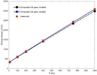
Figure 10 depicts loss curves at various frequencies, determined by assessing the areas under corresponding dynamic loops. This figure illustrates both cases when gexc is constant and as a function of B(t) in the same time αexc is variable. As expected, when choosing the two parameters αexc and gexc as variables in the same time with B(t) the obtained results fit better the measurements. Table 4 shows different values of relative errors with gexc constant and variable at different frequencies. As we can see, the relative errors decrease noticeably when gexc was variable.
The calculation of the relative error is as follows:
$e r r=\frac{\left|E n r_{m e s\,\,\,}-E n r_{c o m\,\,\,}\right|}{E n r_{m e s}} \times 100$ (17)
where, Enrmes and Enrcom are the energy losses measured and computed respectively.
Table 4. Relative errors compared with measurements
|
Frequencies (Hz) |
Relative Errors (%) with gexc Constant |
Relative Errors (%) |
|
200 |
3.27 |
1.08 |
|
400 |
1.89 |
0.76 |
|
750 |
3.79 |
0.90 |
|
1000 |
2.81 |
0.20 |
Figure 10. Computed and measured energy losses with different frequencies
This study introduces a novel approach for accurately modeling hysteresis loop shapes and evaluating energy loss in magnetic materials under high-frequency effects. Through the modification of the excess field expression by employing a new formulation based on magnetic viscosity under high-frequency effects, notable improvements in accuracy and precise predictions compared to measurements have been achieved. The methodology incorporates the consideration of αexc and gexc as variables, dependent on the magnetic flux density, which constitutes a fundamental aspect of our approach. The investigation of the model's behavior encompasses two propositions. The first proposition involves a constant value for gexc and a variable αexc, while the second proposition incorporates variability for both αexc and gexc. The first proposition demonstrates satisfactory hysteresis loop shapes at frequencies below 400 Hz, while the second proposition yields consistent results across different frequency levels. Nonetheless, it is crucial to acknowledge the inherent limitations and uncertainties associated with accurately modeling hysteresis loop shapes, especially when dealing with varying frequencies. The complexity and variability of hysteresis behavior should be duly recognized, prompting the need for further research to fully comprehend these aspects. By acknowledging these limitations, we lay the foundation for future investigations and advancements in the accurate prediction of hysteresis loop shapes across various frequency ranges.
|
Man |
Anhysteretic magnetization, (A.m-1) |
|
Ms |
Saturation, magnetization, (A.m-1) |
|
a,k,c |
Parameters of JA model |
|
H |
Magnetic field, (A.m-1) |
|
B |
magnetic Flux density (T) |
|
Greek symbols |
|
|
α |
Mean field parameter of JA model |
|
δ |
Direction parameter |
|
αexc |
Excess field parameter |
[1] Giraud, A., Bernot, A., Lefèvre, Y., Llibre, J.F. (2017). Measurement of magnetic hysteresis swelling-up with frequency: Impact on iron losses in electric machine sheets. In 2017 IEEE International Workshop of Electronics, Control, Measurement, Signals and their Application to Mechatronics (ECMSM), Donostia, Spain, pp. 1-6. https://doi.org/10.1109/ECMSM.2017.7945864
[2] Zirka, S.E., Moroz, Y.I., Marketos, P., Moses, A.J. (2006). Viscosity-based magnetodynamic model of soft magnetic materials. IEEE Transactions on Magnetics, 42(9): 2121-2132. https://doi.org/10.1109/TMAG.2006.880685
[3] Ducharne, B., Deffo, Y.T., Zhang, B., Sebald, G. (2020). Anomalous fractional diffusion equation for magnetic losses in a ferromagnetic lamination. The European Physical Journal Plus, 135: 1-14. https://doi.org/10.1140/epjp/s13360-020-00330-x
[4] Hamimid, M., Mimoune, S.M., Feliachi, M. (2013). Incorporation of modified dynamic inverse Jiles-Atherton model in finite volume time domain for nonlinear electromagnetic field computation. Journal of Applied Physics, 113(1): 013915. https://doi.org/10.1063/1.4773535
[5] Li, Y., Zhu, L., Zhu, J. (2018). Core loss calculation based on finite-element method with Jiles–Atherton dynamic hysteresis model. IEEE Transactions on Magnetics, 54(3): 1-5. https://doi.org/10.1109/TMAG.2017.2765704
[6] Zhang, B., Gupta, B., Ducharne, B., Sebald, G., Uchimoto, T. (2018). Dynamic magnetic scalar hysteresis lump model based on Jiles–Atherton quasi-static hysteresis model extended with dynamic fractional derivative contribution. IEEE Transactions on Magnetics, 54(11): 1-5. https://doi.org/10.1109/TMAG.2018.2832242
[7] Hamimid, M., Mimoune, S.M., Feliachi, M. (2011). Hybrid magnetic field formulation based on the losses separation method for modified dynamic inverse Jiles–Atherton model. Physica B: Condensed Matter, 406(14): 2755-2757. https://doi.org/10.1016/j.physb.2011.04.021
[8] Podbereznaya, I., Pavlenko, A. (2020). Accounting for dynamic losses in the Jiles-Atherton model of magnetic hysteresis. Journal of Magnetism and Magnetic Materials, 513: 167070. https://doi.org/10.1016/j.jmmm.2020.167070
[9] Jiles, D.C. (1994). Frequency dependence of hysteresis curves in conducting magnetic materials. Journal of Applied Physics, 76(10): 5849-5855. https://doi.org/10.1063/1.358399
[10] Bertotti, G., Fiorillo, F., Soardo, G.P. (1988). The prediction of power losses in soft magnetic materials. Le Journal de Physique Colloques, 49(C8): C8-1915. https://doi.org/10.1051/jphyscol:19888867
[11] Baghel, A.P.S., Kulkarni, S.V. (2014). Dynamic loss inclusion in the Jiles–Atherton (JA) hysteresis model using the original JA approach and the field separation approach. IEEE Transactions on Magnetics, 50(2): 369-372. https://doi.org/10.1109/TMAG.2013.2284381
[12] Zirka, S.E., Moroz, Y.I., Marketos, P., Moses, A.J. (2004). Dynamic hysteresis modelling. Physica B: Condensed Matter, 343(1-4): 90-95. https://doi.org/10.1016/j.physb.2003.08.036
[13] Baghel, A.P.S., Shekhawat, S.K., Kulkarni, S.V., Samajdar, I. (2014). Modeling of dynamic hysteresis for grain-oriented laminations using a viscosity-based modified dynamic Jiles–Atherton model. Physica B: Condensed Matter, 448: 349-353. https://doi.org/10.1016/j.physb.2014.04.012
[14] Belgasmi, I., Hamimid, M. (2020). Accurate hysteresis loops calculation under the frequency effect using the inverse Jiles-Atherton model. Advanced Electromagnetics, 9(2): 93-98. https://doi.org/10.7716/aem.v9i2.1515
[15] Petrun, M., Steentjes, S. (2020). Iron-loss and magnetization dynamics in non-oriented electrical steel: 1-D excitations up to high frequencies. IEEE Access, 8: 4568-4593. https://doi.org/10.1109/ACCESS.2019.2963482
[16] Jiles, D.L., Atherton, D.L. (1986). Theory of ferromagnetic hysteresis. Journal of Magnetism and Magnetic Materials, 61(1-2): 48-60. https://doi.org/10.1016/0304-8853(86)90066-1
[17] Leite, J.V., Sadowski, N., Kuo-Peng, P., Batistela, N.J., Bastos, J.P.A., De Espindola, A.A. (2004). Inverse Jiles-Atherton vector hysteresis model. IEEE Transactions on Magnetics, 40(4): 1769-1775. https://doi.org/10.1109/TMAG.2004.830998
[18] Zirka, S.E., Moroz, Y.I., Marketos, P., Moses, A.J. (2002). Modelling losses in electrical steel laminations. IEE Proceedings-Science, Measurement and Technology, 149(5): 218-221. https://doi.org/10.1049/ip-smt:20020619
[19] Zirka, S.E., Moroz, Y.I., Steentjes, S., Hameyer, K., Chwastek, K., Zurek, S., Harrison, R.G. (2015). Dynamic magnetization models for soft ferromagnetic materials with coarse and fine domain structures. Journal of Magnetism and Magnetic Materials, 394: 229-236 https://doi.org/10.1016/j.jmmm.2015.06.082
[20] Bishop, J.E.L. (1976). The influence of a random domain size distribution on the eddy-current contribution to hysteresis in transformer steel. Journal of Physics D: Applied Physics, 9(9): 1367. https://doi.org/10.1088/0022-3727/9/9/013
[21] Zirka, S.E., Moroz, Y.I., Harrison, R.G., Chwastek, K. (2012). On physical aspects of the Jiles-Atherton hysteresis models. Journal of Applied Physics, 112(4): 043916. https://doi.org/10.1063/1.4747915
[22] Sadowski, N., Batistela, N.J., Bastos, J.P.A., Lajoie-Mazenc, M. (2002). An inverse Jiles-Atherton model to take into account hysteresis in time-stepping finite-element calculations. IEEE Transactions on Magnetics, 38(2): 797-800. https://doi.org/10.1109/20.996206
[23] Jiles, D.C. (1994). Modelling the effects of eddy current losses on frequency dependent hysteresis in electrically conducting media. IEEE Transactions on Magnetics, 30(6): 4326-4328. https://doi.org/10.1109/20.334076
[24] Reinert, J., Brockmeyer, A., De Doncker, R.W. (2001). Calculation of losses in ferro-and ferrimagnetic materials based on the modified Steinmetz equation. IEEE Transactions on Industry Applications, 37(4): 1055-1061. https://doi.org/10.1109/IAS.1999.806023
[25] Chenattukuzhiyil, S. (2015). Study of domain wall dynamics in the presence of large spin-orbit coupling: Chiral damping and magnetic origami. Doctoral dissertation, Universite Grenoble Alpes.