Measurement of Bubbly Two-Phase Flow in a Vertical Pipe Using Ultrasonic Velocity Profiler and Digital Optical Imaging

2.1 Principle of UVP and multiwave UVP methods

The principle of the conventional UVP method is shown in Figure 1 (a). The velocity of moving seeding particles in the flow field is calculated based on the Doppler effect. In the UVP method, the ultrasonic TDX emits a series of ultrasonic pulses into the flow field at a pulse repetition frequency F_prf. After the emission of each pulse, the TDX immediately switches to the receiving mode. Hence, the echo signal from all depths starting from the TDX surface forwards is captured. The maximum depth for the reception of the echo signal corresponds to the maximum time which is set for the receiving mode of the pulser/receiver (P/R) before the next pulse is emitted. As shown in Figure 1, when t_sample-n varies, the positions where the fluid velocity is calculated along a velocity profile are specified. And, the echo signal corresponding to each position is acquired from the whole echo data. The Doppler shift frequency f_d of each position is obtained by processing the digital echo signal at each position. Thus, the fluid velocity at these positions is calculated. Hence velocity profiles of fluid flows are obtained.

1a.png

(a)

1b.png

(b)

Figure 1. The principle of: (a) the UVP method; (b) the multiwave UVP method

Two well-known signal processing algorithms are widely used to calculate f_d. These are Fourier transform-based signal processing that works in the frequency domain and correlation-based signal processing that works in the time domain. These algorithms are implemented in our multiwave UVP system. The behavior of the two algorithms when they are applied to the measurement of two-phase air-water bubbly flow in this study is also evaluated.

When the conventional UVP method for single phase flow measurement is applied to two-phase air-water bubbly flow, ultrasound is not only reflected from seeding particles-ultrasound reflectors but also gets reflected strongly from the bubble-liquid interface. Hence the measured velocity includes the velocity of bubbles as well when bubbles cross the ultrasonic beam. Thus, if we use two ultrasonic frequencies, it is possible to measure separately velocity profiles of each phase. There comes the idea of multiwave UVP method for two-phase flow measurement.

The multiwave UVP method exploits two ultrasonic frequencies [9]. In order to do so, a mutliwave TDX has been developed. The sensor is able to emit and receive two ultrasonic frequencies at the same time and position as shown in Figure 1 (b). The 2 MHz component has a diameter of 10 mm. It has a cylindrical and hollow shape. This sensor is used to measure the bubble phase. The sensor of the 8 MHz frequency has a diameter of 3 mm. This sensor fits in the hollow of the 2 MHz sensor and is exploited to measure the liquid phase. Each sensor is excited and controlled by one independent P/R to emit and receive the ultrasound. The P/Rs are connected with a two-channel data acquisition unit-ADC. The P/Rs and ADC are synchronized as depicted in Figure 1 (b). Received data of each channel is analyzed using the quadrature detection algorithm [6].

2.2 Phase separation in multiwave UVP method

2a.png

(a)

2b.png

(b)

Figure 2. Instantaneous velocity profiles showing: (a) bubble data included in 8MHz data; (b) relative positions of bubbles and the ultrasonic beams

However, an inherent issue of phase separation in two-phase flow measurement must be considered. Similar to the applications of some other measurement methods, such as LDA-Laser Doppler Anemometry, PIV-Particle Imaging Velocimetry methods etc., to the measurement of two-phase flow, the measured data of the liquid phase includes some data of the bubble phase as well. In the multiwave UVP method, it is the inclusion of the velocity of some bubbles in the measured data of the liquid phase by the 8 MHz frequency. In the multiwave UVP method, the 2 MHz frequency can be set to measure only bubble velocity. Phase separation is not needed for the 2 MHz frequency. For the 8 MHz frequency, the problem is schematically shown in Figure 2 (a). A phase separation technique is required to eliminate the bubble velocity from the measured data, Figure 2 (b) [6].

As shown in Figure 2 (b), bubbles will be detected if they appear along the 2 MHz sound path. Using the detected information, the corresponding data of the bubbles included in the 8 MHz frequency is eliminated. Thus, instantaneous velocity profiles of each phase can be measured separately. It is worth noting that, presently, the phase separation is a post-processing procedure that is applied to the stored measured data of each frequency.

2.3 High-speed digital optical imaging and background subtraction

3a.png

(a)

3b.png

(b)

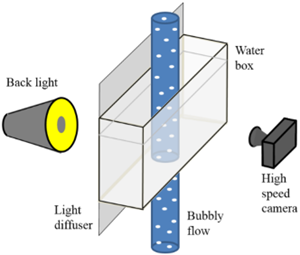
Figure 3. (a) high-speed optical imaging; (b) digital image processing implemented in ImageJ

Shadow images of the bubbly flow are obtained using a high-speed video camera JVC video camera (JVC Hybrid Camera GC-PX1, JVC Co. Ltd.), which is capable of filming the flow images at maximum frame rate 300 fps. At this speed, and with the flow configuration investigated, the effects of the bubble motion in the recorded flow images can be neglected. Visually, it means that negligible bubble streak can be assumed. The arrangement of the light source and the camera is schematically described in Figure 3 (a). A water box is used to eliminate the distortion of the bubble images which is caused by the round shape of the pipe wall. As shown in the bubble image on the left of Figure 3 (b), images with highly contrasted bubbles have been successfully obtained. Note that, for ease of presentation, the photo has been rotated 90 degrees clockwise. In addition, in Figure 3 (b), the position of the multiwave UVP sensor is noted. The location of UVP measurement and that of optical visualization is at the same position along the vertical direction of the flow. The results of optical visualization of the bubble phase in two-phase flow have been extensively investigated in detail previously and confirmed theoretically and experimentally [10, 11].

In each optical visualization, one image of the background flow, i.e., the single phase liquid flow without air bubbles, was taken. Before further digital image processing of the bubble images, preliminary processing of the flow images is carried out, such as background subtraction, region of interest-ROI extraction etc. The image on the right of Figure 3 (b) shows only bubbles in the ROI which is limited to the flow field. Note that the processed image on the right of Figure 3 (b) has been rotated back 90 degrees counter-clockwise to show the vertically upward flow of air bubbles. The macro feature of ImageJ facilitates automatic processing of a large number of images efficiently. During this process, the scale of the images which means the ratio of the number of the pixels (corresponding to the known size of some real object in the image) to the size of the object (usually in mm) is also set. The real size of the objects, i.e., bubbles in this study, detected in the following analyses is calculated using this scale.

2.4 Bubble image analysis algorithm

The objective of digital image processing algorithm in this section is to accurately detect or segment bubbles in bubble images. An example of the resulted image is shown in the right image of Figure 3 (b). For this purpose, widely-used straightforward yet robust thresholding algorithms implemented in the digital image processing tool ImageJ, NIH, USA have been used. The macro is in the form of function calls-scripts in ImageJ macro. To increase the accuracy of the bubble boundary recognition, the threshold for the separation between bubbles and background is carefully selected either based on the image of a known-size object submerged in the flow field or based on automatic thresholding algorithms. As the result, the accuracy of the detection of bubble boundary can be sufficiently high.

In addition, some other image processing algorithms are exploited to improve the quality of the bubble recognition such as hole filling, edge detection etc. [12]. One option is to use the Analyze Particles function of ImageJ which combines the above-mentioned algorithms with adjustable parameters. It is also possible to put a function call to Analyze Particles in an ImageJ macro to facilitate a batch processing of a large number of images. Consequently, individual bubbles are isolated from the bubble images and hence their parameters are available and output to a text file for next analyses. Basically, this is just 2D information.

In the case of bubbly flow, based on theoretical and experimental analyses, the bubble shape can be adequately assumed to have some particular 3D shape, e.g., ellipsoid. Therefore, the bubble surface area which is directly related to the interfacial area concentration in two-phase flow can be obtained. In the same way, the bubble volume, and hence the void fraction of the flow field, can be well calculated accordingly. The surface area of bubbles and void fraction are instantaneous two-phase flow parameters which are of considerable importance in both theoretical and numerical analysis of two-phase flow.

It is worth noting that the limitation of optical visualization and of digital image processing algorithms is that the digital optical imaging method should only be suitable for two-phase flow configurations where we can avoid overlapping of bubbles in the recorded 2D images. Typically, these are low void-fraction bubbly flows, or flows with big isolated bubbles [13-15].

Below is the outline of the ImageJ macro used in this study:

Table 1. ImageJ macro for the digital optical imaging analysis

As shown in Table 1, typical tasks in digital image processing process include:

Batch processing via a for loop-line 9

Background subtraction-line 15

Bubble detection-line 30

Interested readers can find details about these algorithms in ImageJ documentation [13-15].

2.5 Advantages and limitations of the measurement methods exploited

Main advantages of the two measurement methods used in this study can be outlined below. Both methods are non-intrusive, which is critically important in both theoretical study and practical applications. Non-intrusiveness eliminates any possible effects of the measuring probes on the two-phase flow field which is potentially highly affected by the existence of any inserted objects. In practical applications, it is of considerable difficulty to insert measuring probes in any working systems, especially in industrially extreme conditions. Furthermore, both methods can provide spatially-distributed data which is of significant importance in study of fluid flow in general, and of two-phase flow in particular.

Presently, major limitations of the UVP method can appear when the method is applied in practical situations, such as measurement of existing flow systems etc. The reason is that UVP method requires ultrasonic reflectors in the flow field. In working flow systems in practice, ultrasonic reflectors in the fluid flow might be lacking. This problem can be solved by generating cavitation bubbles with the use of a non-intrusive ultrasonic generator [16]. In this technique, careful investigation needs to be carried out regarding the effects of the appearance of cavitation bubbles on the flow characteristics/parameters. Besides, obviously, the digital optical imaging requires an optical window and transparent working fluid in order to capture the flow image. In some practical flow systems, satisfying this requirement might also be difficult.

4.1 Multiwave UVP results

Using the multiwave UVP method, instantaneous velocity profiles of both liquid and bubbles have been measured along the measurement line, i.e., the ultrasound beam which is shown in Figure 3 (b). Two different signal processing algorithms which are the Fourier transform-based algorithm and the correlation-based one have been tested. Theoretically, the correlation-based techniques can be faster since the computation is not as demanding as the Fourier transform-based technique. This is absolutely confirmed by the results of our investigation in this study. Hence, only the results of the correlation-based technique are presented here. It is worth noting that the Fourier transform-based techniques are of interest when we do analyses in the frequency domain.

Figure 5 (a) shows typical instantaneous velocity profiles of liquid and bubbles along the measurement line at a time instant. These profiles show velocity of both liquid and bubbles. Signal processing ensures that only bubble velocity is measured by 2 MHz frequency as shown in Figure 5 (a). Weak echo signal from seeding particles is eliminated from the received signal of the 2 MHz sensor. However, it is clear that, 8 MHz sensor measured velocity of both liquid and bubbles. Hence here is the area where the proposed phase separation technique plays its role.

5a.png

(a)

5b.png

(b)

Figure 5. (a) instantaneous velocity profiles; (b) average profiles

During post-processing, the phase separation technique has been applied to the measured results of the 8 MHz frequency. to eliminate bubble data from measured data of liquid phase. After phase separation, the instantaneous velocity profiles of each phase are obtained. These data are important in both theoretical and experimental analyses of two-phase flow, e.g., for the calculation of the drift velocity which is the velocity difference between the two phases at a point in the flow field. The drift velocity plays an essential role in the Drift-flux CFD model [1, 3].

Besides instantaneous measured results, average velocity profiles of liquid phase (after phase separation) and bubble phase are shown in Figure 5 (b). Since, on average, the flow is statistically axis-symmetric, Figure 5 (b) shows only one-half of the averaged profiles.

4.2 Digital optical imaging and image processing

Figure 3 shows typical images before and after processing using ImageJ. It is confirmed that all bubbles are detected after this processing.

As shown in Figure 6 (c), all bubbles in the bubble image can be detected and located. The instantaneous bubble shape can be well approximated as ellipses in 2D. As a result, instantaneous spatial-averaged void fraction can be estimated based on the number of bubbles and the bubble sizes detected. The time data of the estimated void fraction which is a highly important parameter of two-phase flow is shown in Figure 7 (a). Thus, the time-averaged void fraction of this flow condition can be calculated to be around 3.4%.

6.png

Figure 6. Digital image processing with ImageJ

7a.png

(a)

7b.png

(b)

Figure 7. (a) spatial average of instantaneous void fraction at the measurement position; (b) PDF-probability density function of the bubble size

Based on the analyzed result of the bubble size, the probability density function-PDF of the bubble size distribution can be calculated. For this flow condition, the PDF of bubble size is shown in Figure 7 (b). The PDF exhibits that the bubble size of this flow condition is from about 4 to 7 mm. The average value is about 5 mm.

Such measured results by the optical visualization combined with those of the multiwave UVP method are highly useful for theoretical study of two-phase flows as well as for numerical simulations of two-phase flows using CFD codes.

It would be worth mentioning that the two measurement methods used in the above measurement would work well when the void fraction of the flow is relatively low. Regarding the UVP method, when the void fraction increases, there are a large number of air bubbles along the measurement line, i.e., the sound path. The bubbles might adversely obstruct the sound transmission or severely scatter the echo sound. As for the optical imaging method, obviously, at high void fraction, bubbles overlap in the bubble images. That causes large error in the image processing algorithms.