Manoharan Govindaraj* | Sivakumar Kaliappan | Ganesh Swaminathan
© 2022 IIETA. This article is published by IIETA and is licensed under the CC BY 4.0 license (http://creativecommons.org/licenses/by/4.0/).
OPEN ACCESS
The problem of finding the pattern that deviates from other observation is termed as outlier. The detection of outlier is getting importance in research area nowadays due to the reason that the technique has been used in various mission critical applications such as military, health care, fault recovery, and many. The analysis of functional data and its depth function plays a crucial role in statistical model for detecting outlier. The depth values alone not enough for finding outliers, since all the low depth values not be an outlier. The main problem of using classical model is that it cannot cop up with the high dimensionality of the data This paper proposed a novel technique based on Reproducing Kernel Hilbert Space curve (RKHS) for detecting outliers in functional data. The proposed RKHS model is based on a special Hilbert space curve associated with a kernel so that it reproduces each function in the space to enhance the performance of data depth function. The proposed method uses distance weighted discrimination classification that avoids overfitting the model and provides better generalizability in high dimensions. The kernel depths perform better performances for detection of outlier in a number of artificial and real data sets.
Hilbert space, data depth function, multivariate outlier, functional data and Euclidean distance
The work proposed a novel technique for outlier detection during the analysis of functional data. Outlier detection is performed to find any deviation in normal behavior. An observation that diverges from all other in a sample of pattern on data is termed as Outlier. Since the outliers bias any statistical analysis, outlier detection is important in exploratory analysis process. In the analysis of functional data, outlying properties can be exhibited. Some of the observations have most extreme maximum or minimum values. This may be obtained due to the variability in data measurement or in errors in experimental data. Outlier normally falls under two classes, namely Univariate and Multivariate. Univariate outlier is the one in which the values are distributed over the single feature space. In Multivariate, distribution of values is happened through n-features space. In most of the applications, outliers shown in Figure 1 can be considered as noise otherwise exceptions that should be excluded. In some of the disciplines like physics, economy, machine learning and cyber security etc. detecting outliers is acquiring major importance. The predictions or accuracy of the training model is affected by the outliers due to the occurrence of drastic change in estimation of fitness [1]. It is up to the analyst to make decision about the necessity of including outlier consideration in their context. The process of detecting and analysis of outlier data is termed as outlier mining.
Generally, outliers are defined as, “Given D dimensional Feature space with a set of N data objects, then the expected number of outliers (ω) is found out by considering the top ω data objects that has dissimilarity with respect to the remaining data objects” [2-4]. The outliers are classified into three categories namely, Global outlier, a data object deviates from real data set, Contextual outlier, a data object deviate from the context it is specified, and Collective outlier, a subset of the data objects deviates from the whole data set. Supervised learning and Unsupervised learning are the two basic methodologies used for mining the outliers. Supervised learning is the one in which the outlier detection is implemented based on the labeled example, while in unsupervised learning the labeling is not necessary. Unsupervised Learning based outlier detection mechanisms falls under various categories such as statistical based approach, distance-based approach, deviation based approach and density based approach.
Figure 1. Outliers in datasets
Distance based outlier getting importance when compared to other detection technique since it has dealt mainly based on the non-parametric machine learning approaches. A point outlier in distance based approaches are defined as “A point x is said to be outlier if no more points $\alpha$ in the data sets are at a distance of d or less distance from x”. Detection of the point outliers has implemented as polynomial algorithm or exponential algorithm. But these algorithms have restrictions in terms of two parameters a and d. To overcome these issues, a new definition based on the distance Dk(p) in k-nearest neighbor is defined as, “Given k and n number of data objects, a point x is said to be outlier if no more n-1 points are having maximum distance Dk than p”.
Univariate Outlier detection methodology is inadequate for functional data because the curve values are non-outlying at each time points of observations even though the curve is functional outlier. Multivariate outlier detection methods have some drawbacks due to the following reason. The plotting methods suitable only up to three dimensions [4, 5]. The methods are not robust methods. The procedure is restricted for normal or elliptical samples. To overcome these issues, an approach based on the functional depth is proposed. There are several strategies evolved to find the functional depth of the curve. This paper proposed a novel multivariate methodology which is based on reproducing kernel Hilbert spatial curve for outlier detection of functional data. The proposed methodology decreases the high dimensionality in a large dataset without loss of useful information.
The next section discusses the survey of the Literature and section three discusses the mathematical model of the Reproducing Kernel Hilbert Space (RKHS) curve. The section 4 elaborates the concepts of RKHS by conducting numerical experiments and section 5 concludes.
Outliers can be identified through the parametric and non-parametric approaches. Parametric approach is the one which involve some assumption about underlying normal distribution of feature space while non parametric approach is the one which does not require any assumption. In parametric approach, the outlier can be recognized by finding probability occurrence of the observation otherwise by calculating the deviations from the mean of the observations. The actual distribution of observations is plotted either as normal distribution or log-normal distribution. The underlying distribution cannot be generalized due to the fact that the parameters associated with the distribution, sometimes even the type of the distribution could not be determined previously. By fitting the curve to the data, the parameters of the data could be inferred. The change in the parameters due to the new incoming data will reflect the change in the location of the curve or deformation in shape of the curve is learned. The change in parameter value is identified as Outliers.
Non parametric approach is the one that generates the mapping function without making any assumption. This approach has the benefits of producing high flexibility by fitting the curve to a large number of functional forms, superior power due to weak assumptions about the underlying function and excellent performance in prediction of accuracy of the model. In univariate outlier detection approach, the feature space has dealt with single variables, so that the detection of outlier is obtained by finding the unusual values for a single variable. Multivariate data analysis is required when the data points map to a higher dimensional feature space as follows
$Y(t)=\left[Y^1(t), Y^2(t) \ldots \ldots Y^P(t)\right] \in R^p$ (1)
The main objective of this research paper is to detect the outlier. The outliers can be identified based on the depth function. A depth function D(y, P) is defined as measurement of median or closeness of the curve y to a probability distribution P on the curve. The position of the curve with the respect to center of the data set is measured. Based on the center of the data set, and the position of the curve, the score is calculated.
The four approaches such as density based, distance based, and the subset based learning approaches are involved in the existing outlier detection systems. Probability based model is used in the distribution based approach using the parameters such as mean or Poisson distribution to find the outliers. Distance threshold is considered with the help of Functional Outlier Map (FOM) to detect the outliers in distanced based outlier detection model. Neighbor’s local density is considered in detecting the outlier in density-based outlier based detection model. there are many subset based approaches have been evolved for the detection of outliers. Fraiman et al. [6] proposed a subset based outlier model that involves a new concept in definition of data depth for functional data. The depth function for univariate data points is analyzed and also average of the central observations (1-α)n where 0≤α≤1 namely, trimmed means that constitutes a class of sample estimates from mean to median for functional data is defined. The obtained result achieves good performance in terms of efficiency and robustness.
Cuevas et al. [7] analyzes the level of NOx around the control station using the functional data analysis. In multidimensional space whose dimensions are infinity, let Y be a random variable of functional data. The value of the variable at different discrete times (t1, t2, ... tm) is observed as a set of values y(t1), y(t2) … y(tm). In the closed interval [tmin, tmax] of the observation space. The behavioral characteristic between the levels of NOx is analyzed for working and week days. The sample is analyzed between two estimators such as functional and trimmed standard deviations. The distance based function is proposed in the paper for the detection of outlier.
Febrero et al. [8] proposed a depth-based approach to measure the centrality of the given curve within a group of trajectories for findings functional outlier detection. The performance of the approach is compared with the existing Monto Carlo Methodology using the data set of NOx. The outliers which mask others are detected at each iteration. Sun and Genton [9] proposed tools namely functional boxplot and enhanced functional boxplot for visualization of data and to generalize it. Functional boxplot and enhanced boxplot are implemented on the children growth data set and U.S. precipitation data set and the performance of the outlier detection is simulated based on the statistics techniques. The band depth of ordering from the center outward of a sample curve for functional data is proposed.
Hubert et al. [10, 11] proposed novel numerical and graphical techniques for detection of functional outliers of multivariate functional data. The statistical depth functions and distance measures are observed using P-dimensional vector space. A functional data set consists of n-curves is observed at different set of time points $t_1, t_2, \ldots . t_T$. In multivariate functional data, it is necessary to observe p-dimensional vector of measurements for each curve and each specified time points. A novel statistical distance measurement technique namely bag distance is used to measure the depth function and rank the data. Wenlin et al. [12] proposed a functional directional outlyingness based outlier detection methodology. A framework based on directional outlyingness for both univariate and multivariate functional data on multidimensional domains is introduced. The functional outlyingness is decomposed into two cases magnitude outlyingness and shape outlyingness. The variation in shape of the curve is measured using conventional depth of statistical approach. The similarity between the sequences of the observations is measured using Dynamic Time Warping methodology.
The distance measurement for depth function of univariate data is calculated using different methodology. Integrated square error is one of the methodology in which error is obtained for each principal components of each curve and then integrate the squared value of error. The integrated squared error is checked against the threshold value for detection of outlier. The novel methodology namely squared robust Mahalanobis distance is measured by converting the given curve into p-dimensional vector data and then applies X2 distribution. The outlier is detected if the squared distance is greater than $\mathrm{x}_{0.99, \mathrm{p}}^2$. Multivariate data analysis, uses Mahalanobis distance to measure the observations deviation from the center of the curve. This distance is necessary for calculating Euclidean distance.
3.1 Reproducing Hilbert spaces
A continuous function whose range lies either in two dimensional planar curve or three dimensional space curve on the closed interval [0, 1] in the Euclidean distance space. The Euclidean distance (s) between real valued function is calculated based on the metric space $s: X \times X \rightarrow R$ and the points $x, y, z \in X$ as follows
The function $F$ is said to be continuous one that mapping $f:(X, s) \rightarrow(Y, s)$ at $x_0$, where $x_0 \in X$ for every $\partial>0$ and $\exists \delta>$ 0 , then $s(x, y)<\partial \rightarrow s(F x, F y)<\delta$. A space that is linear which is closed under addition of vector and scalar multiplication is called as vector space $H$.
$x+y=y+z \in H($ commutative property $)$
$x+(y+z)=(x+y)+z \in H($ Associative property $)$
A vector space H is said to be normed space with the norm $\|x\|$ where $x \in H$ is defined on as
$\|x\|=\sqrt{<x-x\rangle}$
An inner product on $H$ over complex field $C$ is a function $<., .>: H \times H \rightarrow C$ with the property of
A Hilbert space is a vector space H with the inner product $\langle u, v\rangle$ defined with norm $\|x\|$ on it is defined by
$|x|=\sqrt{\langle x-x\rangle}$ (2)
that turns H into a complete metric space. Hilbert spaces in finite dimensional space is specified as Real numbers $\mathrm{R}^{\mathrm{n}}$ and Complex number $\mathrm{C}^{\mathrm{n}}$. In infinite dimensional space, Hilbert space is defined as
$\langle u \cdot v\rangle=\int_{-\infty}^{\infty} u(x) \cdot v(x) d x$ (3)
An evaluation function over the Hilbert space functions (F) is represented as a linear function as follows
$L_x: F \rightarrow R$ such that $L_x(f)=f(x), \forall \mathrm{f} \in \mathrm{F}$ (4)
where, $f$ is a bounded linear functional in which $f(x)=<$ $x, m>$ in which $\mathrm{m}$ is defined by $\mathrm{f}$ and has norm $\|\mathrm{f}\|=\|\mathrm{m}\|$.
Reproducing Kernel Hilbert spaces (RKHS).
If a set Y in which all the point evaluations are considered as bounded linear functional in a Hilbert space of Functions, then the space is termed as Reproducing Kernel Hilbert Space (RKHS).
For each $y_i \in Y, Y \in R^n$, the function $L_{y_i}: F \rightarrow R$ such that $L_{y_i}(f)=f\left(y_i\right), \forall \mathrm{f} \in \mathrm{F}$, then according to the definition of RKHS, the function $\left\{L_{y_i}\right\}_{y_i \in Y}$ is said to be bounded. According to Reisz theorem, the set of functions $\left\{k_{y_i}\right\} \subseteq F$ is defined in a way that
$L_{y_i} f=<f, k_{y_i}>, \forall f \in F$ (5)
The function $\mathrm{k}$ is called as reproducing kernel function which is defined over the feature map function $\emptyset: Y \rightarrow F$ such that $\emptyset(x) \rightarrow k_y$ and $k: Y \times Y \rightarrow R$ as
$k(u, v)=<k_u, k_v>=(\emptyset(u), \emptyset(v))$ (6)
where, ky is called the representer of evaluation at y. A space filing curve is the one that performs mapping of N- dimensional space into one dimensional space. It is the curve that proposed as a linear order of pixels by visiting each pixel only once in a multidimensional space.
3.2 Functional data outlier
The multivariate outlier can be detected by estimating the central tendency of the curve. Generally, the multivariate functional median is identified based on the depth and then the deviation of the curve from the center point is calculated by measuring the distance deviated from the curve. Various depth functions are used for identifying the center point of the curve. Sampling is the concept associated with the evaluation. Whenever the point evaluations are continuous, then sampling in functional spaces is essential to ensure the stability of the functional data.
According to Reisz’s lemma, the function has the ability to reproduce the functional values by means of inner product termed as RKHS [13]. The main issue lies in reproducing the functional values. In earlier, Shannon’s theorem proposed a sine function with inner product of L2 as reproducing kernel in RKHS. The functional space is taken as $[-\pi, \pi]$. Nowadays the reproducing is generalized through semi-inner products for Banach spaces. The accurate reconstruction is possible only when sampled data is available. The minimum norm interpolation technique is proposed for RHKS with the benefit of over-sampling that reduces the approximation errors exponentially. Optimal Finite sampling points could be found based on the concept of fixed reproducing kernel [14-20].
The optimal approximation of the linear functions f is produced from a RHKS by considering a class of linear functional. The optimal approximation based on linear function is studied and the function is approximated by finding the nth minimal errors of class of functions characterized by the eigen values.
Let $\delta_x$ is a point evaluation functional that has a unique kernel function $k: Y \times Y \rightarrow R$ defined over $f \in H$ and $x \in$ $Y, K(x,.) \in H$ and we get
$f(x)=\left(f, K\left(x_1, X_2 \ldots X_i\right)\right)_H$ (7)
The above equation states that the functional values of the function f in H can be reproduced using the kernel function. The characteristics of reproducing kernels to be considered are
$K(u, v)=(\emptyset(u), \emptyset(v))_{H, \text { and u, v $\in$ Y}}$
Two classes of functional data classes such as polynomial and exponential RKHS are proposed. The polynomial classes is specified through the equation
$K(u, v)=\sum_{m=0}^{m=\infty} a_m(u . v)^m, \quad u, v \in R^d$ (8)
where, $\left\{a_m\right\}$ denotes a sequence of non negative number of the kernel series of polynomial class. The series of the numbers that converges for all the functional values $u, v \in R^d$.
Procedure Outlier_ detection
1. Select a functional space for sampling is RKHS. Optimal sampling points are obtained by applying the following procedure
$\overline{f(x)}=\sum_{\mathrm{j}=1}^{\mathrm{m}} \alpha_{\mathrm{j}} \mathrm{k}\left(\mathrm{x}_{\mathrm{j}}, \mathrm{x}\right), \mathrm{x} \in \mathrm{Y}$
where the coefficients $\alpha_j, 1 \leq j \leq m$, are the solutions of
$\sum_{\mathrm{j}=1}^{\mathrm{m}} \alpha_{\mathrm{j}} \mathrm{k}\left(\mathrm{x}_{\mathrm{j}}, \mathrm{x}_{\mathrm{k}}\right)=\mathrm{f}\left(\mathrm{x}_{\mathrm{k}}\right)$
2. The error estimates using the function
3. Obtain optimized sample points $S_{o p t}$ and compare it with the equalized sample points $S_{e q u}$
4. Distance of each point from the optimized sample point of the curve is measured. If there are more deviations then that point is considered to be outlier.
5. Stop
3.3 Procedure for Outlier detection
The steps shown above describes the procedure for Generally, Outliers occur at the low probability region of the stochastic model, inliers occur at the high probability region. The number of sampling points m is fixed. The reconstruction RKHS and the approximation error measurement are the two factors that constitute the mechanisms of selecting the sampling points. According to the Gaussian Reconstruction kernel
$k_\sigma(u, v)=\exp \left(\frac{\|u-v\|^2}{\sigma}\right), u, v \in R^d$ (9)
where, $\sigma>0$ and $\|$.$\|$ denotes a standard Euclidean norm on higher dimensional space. The general form of reconstruction error is constructed as minimization problem as follows
$\min \int_\omega^u \operatorname{distance}{ }^2(K(u, .), \delta) d \mu(u)$
where, $\delta$ refers to subspace in n-dimensional space and $\mu$. Is variation on measurement space. The procedure for outlier detection is shown in Figure 2.
Figure 2. Three heat sources
4.1 Numerical experiments
All the data points from the multidimensional space is transformed into uni-dimensional data points in order to identify the outliers This concept is implemented by finding the distance between two points using Euclidean distance. The performance is further improved by considering the nearest neighbor up to k. Distance vector that consists of distance information for k-neighbors is the right choice for calculating the right outliers. According to the normal distribution, the points below the T is termed as outliers where T is defined as follows
$T=\operatorname{argmax}\left(\sum_{i=1}^n f\left(x_i, y_i\right)\right)$ (10)
where, n denotes the total number of observations and f(x,y) is defined as
$f(x, y)=\frac{1}{2 \pi \beta d_{Q 3}} e^{-\frac{\left(x-x_i\right)^2+\left(y-y_i\right)^2}{2 \beta d_{Q 3}}}$ (11)
where, $\beta$ represents a constant and $d_{Q 3}$ denotes the third quartile. According to the k-closest neighbor the function f(x,y) is defined as
$f(x, y)=\frac{(\delta)^2}{\pi} e^{-\frac{\left(x-x_i\right)^2+\left(y-y_i\right)^2}{\delta^2}}$ (12)
$\delta=\left(\gamma /\left(1+d_k\right)^2\right)^2$ (13)
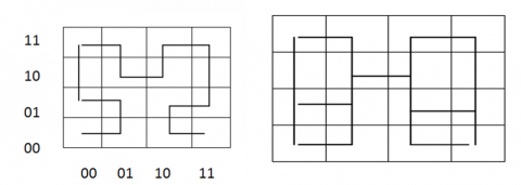
Table 1 discusses the mapping of multidimensional data to a single dimensional data and the corresponding Hilbert curve in Figure 2 and 3.
Table 1. Mapping of N-dimensional space to one dimensional
|
n-d |
1-d |
n-d |
1-d |
n-d |
1-d |
n-d |
|
(00, 00) |
0000 |
(01,00) |
0001 |
(10, 00) |
1110 |
(11,00) |
|
(00, 01) |
0011 |
(01,01) |
0010 |
(10, 01) |
1101 |
(11,01) |
|
(00,10) |
0100 |
(01,10) |
0111 |
(10,10) |
1000 |
(11,10) |
|
(00,11) |
0101 |
(01,11) |
0110 |
(10,11) |
1001 |
(11,11) |
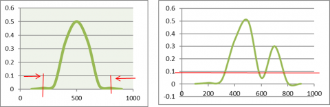
(a) (b)
Figure 3. Gaussian Estimation Model a) Points with critical values that used to decide outliers b) Points that designated as outliers based on the boundaries
4.2 Analysis of proposed methodology
The performance of the proposed approach is analyzed with the help of different datasets using MAT LAB 14.1, Intel Processor. The Univariate datasets PenDigits with samples of 6870, 2.27% outliers, 16 number of features, MNIST datasets with samples of 7603, 9.2% outliers, 100 number of features have taken for analysis. The Multivariate dataset Wine Quality with 7 classes of data with outlier percentage ranges from 0.1% to 44.49% has taken. The detection rate and the detection accuracy is considered to be the parameters for analysis of the proposed methodology is calculated as follows
Detection rate $(D R)=(1-F N R) \times T N R$
Detection Acc $=(D R) / O_{\text {actual }} \times 100$
where
$\begin{aligned} \text { False Negative Rate }(F N R) &=\frac{\text { False Negatives }}{\text { True Positives }+\text { False Negatives }} \\ \text { True Negative Rate }(T N R) &=\frac{\text { True Negatives }}{\text { False Positives }+\text { True Negatives }} \end{aligned}$
The proposed model RKHS curve model is compared with the existing Modified Hidden Markov Model (MHMM), Hidden Semi Markov Model (HSMM) for outlier detection rate and detection accuracy as shown in Figure 4.
(a) (b)
Figure 4. Detection Rate a) Univariate b) Multivariate
It can be observed from the Figure 4.a) that the detection rate of proposed methodology produces better outlier detection rate compared with the existing models Modified Hidden Markov Model and Modified Semi Markov Model. The RKHS model produces a detection accuracy that nearest to the actual outlier percentage.
(a) (b)
Figure 5. Detection Accuracy a) Univariate b) Multivariate
It can be observed from the Figure 5, the detection accuracy of the proposed technology is high compared to the existing MHMM and MSMM. The improvement in detection of outlier accuracy leads to the corresponding improvement in classification accuracy of the system.
In data analytics, the detection of outliers plays an important role for preprocessing the task. Most of the existing approaches for outlier detection needs huge amount of data points to work in an efficient way. It is very difficult to detect the outlier using few data points and they require huge computational cost for high dimensional data. The main benefit of the proposed work is that the approach need not have any distributed assumptions. The performance of the proposed work is evaluated with simulated datasets over the existing Modified Hidden Markov Model (MHMM), Hidden Semi Markov Model (HSMM) for outlier detection rate and detection accuracy When compared to other state-of-art, the proposed techniques based on RKHS produces more accuracy and less cost for computation. The performance of RKHS for Univariate and Mutivariate outlier detection is verified experimentally and compared with existing models MHMM and MSMM. The performance parameters detection rate and detection accuracy are obtained and came to the conclusion that RKHS produces accuracy approximately equal to the actual outlier detection accuracy. The proposed technique is feasible and produces good performance in outlier detection irrespective of data size and the number of dimensions used.
[1] Modarres R. (2011) Data Depth. In: Lovric M. (eds) International Encyclopedia of Statistical Science. Springer, Berlin, Heidelberg. https://doi.org/10.1007/978-3-642-04898-2_201
[2] Angiulli, F., Pizzuti, C. (2002) Fast Outlier Detection in High Dimensional Spaces. In: Elomaa T., Mannila H., Toivonen H. (eds) Principles of Data Mining and Knowledge Discovery. PKDD 2002. Lecture Notes in Computer Science (Lecture Notes in Artificial Intelligence), vol 2431. Springer, Berlin, Heidelberg. https://doi.org/10.1007/3-540-45681-3_2
[3] Liu, R.Y., Serfling, R. (2006). Depth functions in nonparametric multivariate inference. DIMACS Series in Discrete Mathematics and Theoretical Computer Science, 72. https://doi.org/10.1090/dimacs/072/01
[4] Leys, C., Delacre, M., Mora, Y.L., Lakens, D., Ley, C. (2019). How to classify, detect, and manage univariate and multivariate outliers, with emphasis on pre-registration. International Review of Social Psychology, 32(1): 5. http://doi.org/10.5334/irsp.289
[5] Amovin-Assagba, M., Gannaz, I., Jacques, J. (2022). Outlier detection in multivariate functional data through a contaminated mixture model. Computational Statistics & Data Analysis, 174: 107496. https://doi.org/10.1016/j.csda.2022.107496
[6] Fraiman, R., Muniz, G. (2001). Trimmed means for functional data. TEST: An Official Journal of the Spanish Society of Statistics and Operations Research, 10: 419-440. https://doi.org/10.1007/BF02595706
[7] Cuevas, A., Febrero-Bande, M., Fraiman, Ri. (2007). Robust estimation and classification for functional data via projection-based depth notions. Computational Statistics, 22: 481-496. https://doi.org/10.1007/s00180-007-0053-0
[8] Febrero, M., Galeano, P., González-Manteiga, W. (2007). Outlier detection in functional data by depth measures, with application to identify abnormal NOx levels Envi-Ronmetrics: The Official Journal of the International Environmetrics Society, 19(4): 331-345. https://doi.org/10.1002/env.878
[9] Sun, Y., Genton, M.G. (2011). Functional boxplots. Journal of Computational and Graphical Statistics, 20(2): 316-334. https://doi.org/10.1198/jcgs.2011.09224
[10] Hubert, M., Rousseeuw, P., Segaert, P. (2015). Multivariate functional outlier detection. Statistical Methods and Applications, 24: 177-202. https://doi.org/10.1007/s10260-015-0297-8
[11] Hubert, M., Rousseeuw, P., Segaert, P. (2017). Multivariate and functional classification using depth and distance. Advances in Data Analysis and Classification, 11(3): 445-466. https://doi.org/10.1007/s11634-016-0269-3
[12] Dai, W.L., Genton, M.G. (2019). Directional outlyingness for multivariate functional data. Computational Statistics & Data Analysis, 131: 50-65. https://doi.org/10.1016/j.csda.2018.03.017
[13] Angelin, B., Geetha, A. (2020). Outlier detection using clustering techniques-K-means and K-median. In: Proceedings of the International Conference on Intelligent Computing Control System (ICICCS), pp. 373-378. https://doi.org/10.1109/ICICCS48265.2020.9120990
[14] Bergman, L., Hoshen, Y. (2020). Classification-based anomaly detection for general data. arXiv.
[15] Wahid, A., Annavarapu, C.S.R. (2021). NaNOD: A natural neighbour-based outlier detection algorithm. Neural Comput. and Appl., 33: 2107-2123. https://doi.org/10.1007/s00521-020-05068-2
[16] Domański, P.D. (2020). Study on statistical outlier detection and labelling. Int J Autom Comput., 17: 788-811. https://doi.org/10.1007/s11633-020-1243-2
[17] Dong, Y., Hopkins, S.B., Li, J. (2019). Quantum entropy scoring for fast robust mean estimation and improved outlier detection. arXiv.
[18] Shetta, O., Niranjan, M. (2020). Robust subspace methods for outlier detection in genomic data circumvents the curse of dimensionality. R Soc Open Sci., 7(2): 190714. https://doi.org/10.1098/rsos.190714
[19] Lim, P., Niggemann, O. (2020). Non-convex hull based anomaly detection in CPPS. Eng Appl Artif Intell., 87: 103301. https://doi.org/10.1016/j.engappai.2019.103301
[20] Borghesi, A., Bartolini, A., Lombardi, M., Milano, M., Benini, L. (2019). Anomaly detection using autoencoders in high performance computing systems. CEUR Workshop Proc., 2495: 24-32. https://doi.org/10.48550/arXiv.1811.05269