Bachir Selmoune | Mourad Hamimid*
© 2021 IIETA. This article is published by IIETA and is licensed under the CC BY 4.0 license (http://creativecommons.org/licenses/by/4.0/).
OPEN ACCESS
In this paper, an accurate evaluation of minor hysteresis loops using the modified Jiles-Atherton model is presented. This model is based on the anhysteretic magnetization, which is given in most cases by the Langevin equation. The anhysteretic magnetization is characterized by three parameters, the mean field parameter α, the shape parameter of anhysteretic magnetization curve a and the saturation magnetization Ms. The parameters influencing the minor hysteresis loops are a and α. These parameters are expressed usually in the form of simple power laws and they connect the minor loop parameters to the major ones. These expressions are applicable in both centered and non-centered minor loops cases. In the centered minor loops, the parameter k is introduced in order to adjust the width of the minor loops regarding the level of the magnetic excitation. The coefficients of the proposed expressions (γ, β and σ) are obtained by optimization procedure. The proposed approach is validated using measured minor loops in both cases. A close agreement is obtained between modeled and measured ones.
anhysteretic magnetization, non-centered minor loops, centered minor loops, Jiles-Atherton hysteresis model, Identification
The principal objectives in modeling magnetic materials are based on the magnetic properties of the ferromagnetic materials. To describe with accuracy the real physical behavior of the magnetic cores used in the electrical energy conversion, several precise models have been proposed in the literature. Among these models which represent the hysteresis phenomenon characteristic, the Preisach model, the Jiles–Atherton model [1, 2], Stoner–Wolfarth model [3, 4], and the Mayergoyz model [5]. The Jiles-Atherton model (JA) is the widely used one, and it has proved its efficiency in many applications However, the JA model has a major drawback in describing the minor loops. Recently, more important papers have been published, aimed at better representation of minor hysteresis loops [6-10].
In this work, we deal with a solution to the problem that is often addressed by researchers, especially in references [6-10]. First, when the hysteresis loops model operates at low flux density levels, the JA model gives a poor representation of centered minor hysteresis loops and exhibits a certain unphysical behavior [6, 7].
Secondly, the use of power electronics converters generates harmonics in electrical systems, these harmonics cause non-centered minor hysteresis loops which leads to increase the iron losses, the JA model cannot predict the iron losses in such situations [8, 9], Many researchers have suggested several ways to improve the JA model, for instance in ref. [6, 7], the researcher proposed a modification of three model parameters (a, α, and k) in order to improve the centered minor hysteresis loops, accurate results are obtained but the comparison was limited to the centered minor loops only. In ref. [8], the researcher proposed a modification of four model parameters (a, α, c and k) in order to improve the non-centered minor loops, also, in ref. [9] the researcher proposed a modification of the parameters c and k according to the variation of the magnetic field, and acceptable results are obtained for the non-centered minor hysteresis loops, without testing the case of the centered mirror loops. In the work of Ref [10], the high-variation rate of the irreversible magnetization, which causes the non-physical behavior of minor loops, is limited by introducing a new physical parameter ‘R’ linked to the losses. The proposed approach gives accurate results in both cases centered and non-centered minor loops but the process needs several measurements in order to identify the parameter ‘R’.
We can use another alternative to improve JA model representation for minor hysteresis loops in both centered and non-centered minor loops cases. Depending on the foregoing and since there is no way to change the values of anhysteretic magnetization except by changing its parameters; we consider the value of the saturation magnetization to be constant. Therefore only two model parameters should be evaluated for the minor loops which are directly related to the anhysteretic magnetization.
These parameters are evaluated by using judicious expressions, based on simple power laws, which are applicable in both centered and non-centered minor loops cases. Similar functional dependences of minor loops parameters have been the subject of intensive research [11, 12]. In the case of the centered minor hysteresis loops the parameter k is introduced to adjust the width of the minor hysteresis loops, when the level of the magnetic excitation increases. These expressions are identified using an optimization procedure which minimizes the error between the measured and calculated hysteresis loops.
In the original Jiles–Atherton (JA) model, the total magnetization is decomposed into reversible component Mrev, representing the translation and the reversible rotation of the walls with in ferromagnetic materials, and their reversible component Mirr which corresponds to domain wall displacement against the pinning effect, M= Mrev +Mirr. This usually used model is formulated in terms of a set of equations having five parameters. The original JA model allows the computation of the magnetic induction from the known magnetic field as independent variable. However, in some calculation procedures the induction is known before the field. to achieve such simulations, a modified JA model presenting the magnetic induction as independent variable. The modified inverse Jiles Atherton model (MIJA) considering the magnetic flux density as an independent variable is given as [13].
$\frac{d M}{d B}=\frac{k \delta c \frac{d M_{a n}}{d H_{e}}+\left(M_{a n}-M\right)}{\mu_{0}\left(k \delta+(1-\alpha)\left(k \delta c \frac{d M_{a n}}{d H_{e}}+\left(M_{a n}-M\right)\right)\right)}$ (1)
where the effective field,
$H_{e}=H+\alpha M$ (2)
The anhysteretic is given by:
$M_{a n}=M_{s}\left(\operatorname{coth} \frac{H_{e}}{a}-\frac{a}{H_{e}}\right)$ (3)
And
$\frac{d M_{a n}}{d H_{e}}=\frac{M_{s}}{a}\left(1-\left(\operatorname{coth}\left(\frac{H_{e}}{a}\right)\right)^{2}-\left(\frac{a}{H_{e}}\right)^{2}\right)$ (4)
a, α, c, k and the saturation magnetization Ms are the five model parameters which have to be determined from measured major hysteresis loops; δ is a directional parameter taking the value 1 for dB/ dt > 0 and -1 for dB /dt < 0.
In this work the calculation is performed using 3% Fe–Si non-oriented magnetic sheets. These sheets are characterized by 0.5 mm thick laminations [6, 7], The MIJA model is characterized by five parameters and in most cases, and they are identified using a major hysteresis loop. These five parameters are given in ref. [10] and they are presented in Table 1.
Table 1. Model parameters under sinusoidal wave-form flux density [10]
|
Parameters of model |
Values |
|
Ms (A/m) |
1.58×10⁶ |
|
a (A/m) |
105 |
|
k (A/m) |
57.3 |
|
$\alpha$ (-) |
2×10⁻⁴ |
|
c (-) |
0.27 |
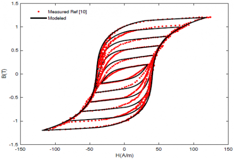
Figure 1 shows a comparison between measured and modeled hysteresis loops with JA model, by using the model parameters obtained from the major loop and they are presented in Table 1.
As expected, when the model operates near the saturation flux density, the measured and modeled hysteresis loops are in good agreement.
On the other hand, when the model operates at low flux density levels less than the saturation, the model does not fit the measured ones and the discrepancies between measured and modeled hysteresis loops is significant.
Figure 1. Measured and modeled centered minor hysteresis loops (Bmax =0.2 T to 1.2T, step 0.2T)
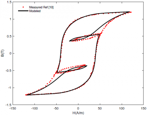
When the flux density contains harmonics, the model of JA does not able to represent the non-centered minor hysteresis loops by using the same parameters presented in Table 1.
In fact, the magnetization in the non-centered minor loop requires an additional time to pass through the first turning point, and there is no condition ensuring the passage through the initial point when the minor loop is achieved. Figure 2 shows modeled and measured hysteresis loops include non-centered ones.
Figure 2. Measured and modeled hysteresis loops under non-sinusoidal waveform flux density
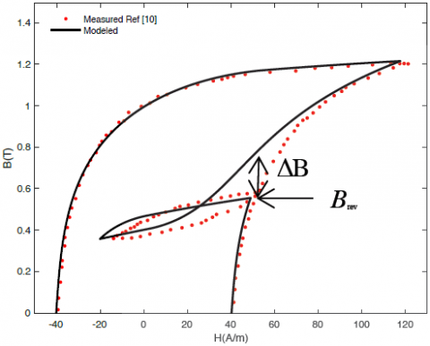
Figures 1-2 show the drawbacks of JA model in presence of minor loops. This non-physical behavior reduces the uses of the model in the case of low flux density levels, or when the excitation contains harmonics. Figure 3 shows the zoom-up to the modeled and measured hysteresis loops under non-sinusoidal waveform flux density. It is clearly noted that the non-centered minor hysteresis loop is non-closure. One can also observe that the flux density is too high (ΔB) during the closure of the minor loop.
Figure 3. Measured and modeled hysteresis loops under non-sinusoidal waveform flux density (zoom at turning point)
The JA model is established at first on the anhysteretic magnetization, the latter is given in most cases by the Langevin equation (Eq. (3)), and it is characterized by three parameters, the mean field parameter α, the shape parameter of anhysteretic magnetization curve a, and the saturation magnetization Ms.
In this work, a modification of anhysteretic magnetization is achieved by modifying their parameters. These parameters are related to the major ones and the ratio between the reverse flux density Brev for the minor loop and the saturation flux density Bsat of the major hysteresis loop.
The determination of Brev value is very easy in the case of the centered minor loops (Brev=Bmax), however, in the non-centered minor loops case, one can identify Brev at the turning points by the observation of the directional parameter δ, if (δ=+1) the magnetization is on its ascendant branch else on its descendant branch (δ=-1), the change in the value of δ indicates that the reversible point is achieved, in this moment the value of Brev is recorded.
For the non-centered model, the main parameters influencing the minor hysteresis loops are the shape parameter of anhysteretic magnetization curve a and the mean field parameter α, and they are given by Eqns. (5) and (6).
$a_{\min }=a_{m a j}\left(\frac{B_{r e v}}{B_{\text {sat }}}\right)^{\gamma}$ (5)
$\alpha_{\min }=\alpha_{\operatorname{maj}}\left(\frac{B_{\text {rev }}}{B_{\text {sat }}}\right)^{\beta}$ (6)
amin and αmin represent the minor hysteresis loop parameters. amaj and αmaj represent the major ones and they are given in Table 1.
We also recall that; the width of the centered minor loops increases with magnetic excitation levels. It has been mentioned that for very soft magnetic materials, the pinning parameter k is proportional to the width of the hysteresis loop [14, 15]. Therefore, to adjust the width of the centered minor loops, the parameter k should be modified with the same aforementioned procedure, as follows:
$k_{\min }=k_{\operatorname{maj}}\left(\frac{B_{r e v}}{B_{s a t}}\right)^{\sigma}$ (7)
The coefficients γ, β and σ are constants to be determined by an optimization procedure which minimizes the error between measured and calculated hysteresis loops.
Eq. (8) shows the objective function to be minimized, based on the quadratic error between measured and modeled magnetic field.
$e r r=\frac{\sqrt{\sum_{i}^{N}\left(H_{\text {meas }}^{i}-H_{\text {mod }}^{i}\right)}}{N}$ (8)
N is number of measured points, Hmeas and Hmod are respectively the measured and the modeled magnetic field.
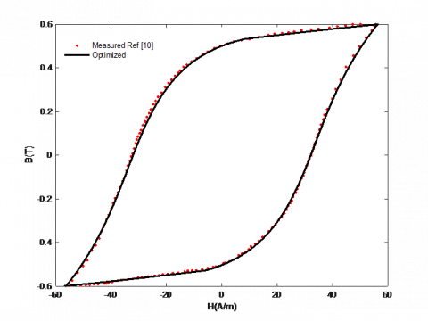
The coefficients γ, β and σ are optimized once by using the Pattern Search (PS) in MATLAB Optimization tools, for the measured flux density Bmax=0.6 T. The optimized coefficients are presented in Table 2. The respective values of the model parameters were updated to amin=130.98 Am-1, amin=2.20 ´10-4 and kmin=44.92 Am-1. The comparison between the measured and the optimized minor hysteresis loops shows a good agreement (Figure 4).
Figure 4. Optimized and measured minor hysteresis loop (Bmax = 0.6 T)
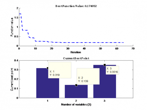
Figure 5 shows the quadratic error between measured and modeled magnetic field, and shows also the best obtained value of the three coefficients γ, β and σ.
Figure 6 shows the variation of the normalized, k/kmax, a/amax and a/amax versus Brev, with kmax=57.3(A/m), amax= 189.72 (A/m) and amax=2.63×10⁻⁴
By using the set of coefficients presented in Table 2, we determine the parameters a, a and k by using Eqns. (5), (6) and (7) for any arbitrary maximum flux density. Figure 7 shows the centered minor hysteresis loops obtained after the model parameters modification. The modeled hysteresis loops fitted the measured ones compared to the results presented above in Figure 1.
Figure 5. Quadratic error and the best obtained coefficients at (Bmax = 0.6 T)
Table 2. The optimized coefficients
|
Coefficients |
Values |
|
g |
-0.319 |
|
b |
-0.139 |
|
σ |
0.351 |
Figure 6. Variation of the three parameters versus Brev
In order to show the effectiveness of the proposed approach, the volumetric energy density dissipated per unit volume is calculated in both cases, model with and without modification. The volumetric energy density is expressed as an integral over the loop and is given as:
$W=\int_{0}^{B} H d B$ (9)
Figure 8 presents the obtained volumetric energy density (Joule/m3) in both cases compared with measurements.
We can see clearly that the obtained volumetric energy density by the proposed model fit better the measurements ones compared to the volumetric energy calculated by the model without modification. Figure 9 shows a comparison between measured and modelled non-centred minor hysteresis loops, in this case the modification is made only for two parameters a and α, i.e. the anhysteretic magnetization parameters. The obtained results depicted in Figure 9 show clearly that the non-centered minor loops are completely closed, and they are in good agreement with measurements.
Figure 7. Measured and modeled centered minor loops (Brev=Bmax = 0.2 T to 1.2 T, step 0.2 T)
Figure 8. Measured and calculated dissipated energy density
Figure 9. Measured and modeled non-centered minor loops under non-sinusoidal waveform flux density
In order to show clearly the closure of the non-centered minor loop, Figure 10 shows a zoom-up at turning point, it can clearly be seen that the results are considerably improved by modifying only two parameters, compared to those shown above in Figure 3.
Figure 10. Zoom-up, measured and modeled non-centered minor hysteresis loops
An accurate evaluation of the minor hysteresis loops is proposed by modifying the anhysteretic magnetization parameters. The main idea is based on considering that the anhysteretic magnetization parameters are given by appropriate expressions. These expressions have a simple power law. The modified minor loops parameters are depending on the major ones and the ratio between saturation flux density of the major hysteresis loop and the reversible flux density of the minor ones. This approach is applied in both, centered and non-centered, minor loops. The improvement of the JA model makes it more useful for future applications.
|
Man |
anhysteretic magnetization |
|
a, k,c, Ms |
Parameters of JA model |
|
H |
magnetic field, A/m |
|
B |
flux density, T |
|
W |
volumetric energy density m, Joule/m3 |
|
Greek symbols |
|
|
$\gamma, \beta, \sigma$ |
constants determined by an optimization procedure |
|
$\alpha$ |
mean field parameter of JA model |
[1] Füzi, J. (2004). Two Preisach type vector hysteresis models. Physica B: Condensed Matter, 343(1-4): 159-163. http://dx.doi.org/10.1016/j.physb.2003.08.089
[2] Jiles, D.C., Atherton, D.L. (1986). Theory of ferromagnetic hysteresis. J. Magnetism and Magnetic Materials, 61(1-2): 48-60. http://dx.doi.org/10.1016/0304-8853(86)90066-1
[3] Chuev, M.A., Hesse, J. (2007). Nanomagnetism: Extension of the Stoner– Wohlfarth model within Néel's ideas and useful plots. Phys: Condens. Matter, 19(50): 506201. http://dx.doi.org/10.1088/0953-8984/19/50/506201
[4] Tannous, C., Gieraltowski, J. (2008). The Stoner–Wohlfarth model of ferromagnetism. Eur. J. Phys., 29: 475-487. http://dx.doi.org/10.1088/0143-0807/29/3/008
[5] Mayergoyz, I.D. (2003). CHAPTER 4 - stochastic aspects of hysteresis. Mathematical Models of Hysteresis and Their Applications, 225-297. https://doi.org/10.1016/B978-012480873-7/50005-0
[6] Hamimid, M., Mimoune, S.M., Feliachi, M. (2013). Evaluation of minor hysteresis loops using Langevin transforms in modified inverse Jiles– Atherton model. Physica B: Condensed Matter, 429: 115-118. http://dx.doi.org/10.1016/j.physb.2013.08.014
[7] Hamimid, M., Mimoune, S.M., Feliachi, M. (2012). Minor hysteresis loops based on exponential parameters scaling of the modified Jiles- Atherton model. Physica B: Condensed Matter, 407(13): 2438-2441. http://dx.doi.org/10.1016/j.physb.2012.03.042
[8] Hamimid, M., Mimoune, S.M., Feliachi, M., Atallah, K. (2014). Non centered minor hysteresis loops evaluation based on exponential parameters transforms of the modified inverse Jiles–Atherton model. Physica B: Condensed Matter, 451: 16-19. http://dx.doi.org/10.1016/j.physb.2014.06.021
[9] Benabou, A., Leite, J.V., Clénet, S., Simao, C., Sadowski, N. (2008). Minor loops modelling with a modified Jiles-Atherton model and comparison with the Preisach model. J. Magnetism and Magnetic Materials, 320: 1034-1038. http://dx.doi.org/10.1016/j.jmmm.2008.04.092
[10] Leite, J.V., Benabou, A., Sadowski, N. (2009). Accurate minor loops calculation with a modified Jiles Atherton hysteresis model. COMPEL, 28(3): 741-749. http://dx.doi.org/10.1108/03321640910940990
[11] Chwastek. K. (2009). Modelling offset minor hysteresis loops with the modified Jiles-Atherton description. J. Phys. D: Appl. Phys., 42(16): 165002. http://dx.doi.org/10.1088/0022-3727/42/16/165002
[12] Chwastek, K., Szczygłowski, J. (2009). Modelling dynamic hysteresis loops in steel sheets. COMPEL, 28(3): 603-612. http://dx.doi.org/10.1108/03321640910940873
[13] Hamimid, M., Feliachi, M., Mimoune, S.M. (2010). Modified Jiles-Atherton model and parameters identification using false position method. Physica B: Condensed Matter, 405(8): 1947-1950. http://dx.doi.org/10.1016/j.physb.2010.01.078
[14] Jiles, D.C., Thoelke, J.B., Devine, M.K. (1992). Numerical determination of hysteresis parameters for the modeling of magnetic properties using the theory of ferromagnetic hysteresis. IEEE Trans. Magn., 28(1): 27-35. http://dx.doi.org/10.1109/20.119813
[15] Jiles, D.C., Thoelke, J.B. (1989). Theory of ferromagnetic hysteresis: determination of model parameters from experimental hysteresis loops. IEEE Trans. Magn., 25(5): 3928-3930. http://dx.doi.org/10.1109/20.42480