Reham A. Eltuhamy* | Mohamed Rady | Khaled H. Ibrahim | Haitham A. Mahmoud
© 2020 IIETA. This article is published by IIETA and is licensed under the CC BY 4.0 license (http://creativecommons.org/licenses/by/4.0/).
OPEN ACCESS
Regarding the fault diagnosis of Copper Indium Gallium Selenide (CIGS) PV modules, previously published articles focused on employing statistical analysis of thermography images. This approach failed in many cases to distinguish among fault types. This article presents a novel methodology to diagnose and predict faults of thin-film CIGS PV modules using infrared thermography analysis combined with measurements of I-V characteristics. The proposed methodology encompasses a comprehensive site work to capture images that cover many fault types of the PV module under study. The novelty of the technique depends on utilizing processing and analysis of the captured images using new proposed mathematical parameters to extract different faults’ features. Using I-V measurements combined with thermography analysis, the differences between different types of faults are detected. Then, a general classification matrix of CIGS fault detection and diagnosis, using features based on mathematical parameters and IV measurements has been established. Results show that the analysis of the temperature distribution is proved to be insufficient to identify specific modes of different faults. In addition, the proposed procedure for fault detection and classification, which depends on the pattern of faults, can be used for any type of PV module. This results in more reliance on the proposed technique to increase the confidence level of fault detection.
PV, CIGS, fault classification, thermography, IV, fault detection, features extraction, mathematical parameters
Power generation from solar PV is continuously increasing all over the world. In 2018, a 30% increase in PV energy production corresponding to 570 TWh has been recorded. In 2018, the increase in solar PV capacity additions globally reached 97 gigawatts (GW) corresponding to around half of total net renewable capacity growth. Solar PV capacity additions have been doubled from 2016 to 2017 [1]. The common photovoltaic module (PVM) technologies include; Monocrystalline silicon PV modules, Polycrystalline silicon PV modules, Amorphous silicon PV modules, and Thin-film PV modules. Even though monocrystalline silicon PV and polycrystalline silicon PV are used more than other technologies, the thin-film module production grows at the rate of 24% from 2009 to reach 22,214 MW production by 2020. One type of thin-film technology is CIGS which is getting more popular than different thin-film technologies because of its higher efficiency and reduced manufacturing costs. The success of CIGS cells is supported by continuous improvement in efficiency, faster and cheaper manufacturing processes, and favorable payback time.
The rapid development of solar energy applications in residential, commercial, and industrial sectors is making photovoltaic energy an integral component of new green facilities. To achieve high performance, efficiency, and reliability of photovoltaic plants, the early detection of PV faults is recommended. One of the most effective techniques is the infrared thermography method (IRT), as it provides fast, contactless, nondestructive, and real-time fault detection and diagnosis (FDD). The early studies that investigate the detection of photovoltaic faults using IRT are addressed in the studies [2-4].
The factors that should be carefully considered while using thermography measurements for photovoltaic modules in the outdoor conditions include qualified personnel, emissivity adjustment, distance of the object being inspected, angle of capturing, and ambient meteorological conditions [5-9]. Field IR imaging of PV modules provides a useful tool to identify different PV faults via the analysis of their thermal effects. The infrared image of the faulty module has thermal signatures that appear as regions with different temperatures in the captured image. However, these effects are difficult to interpret without careful anslysis of the interconnection between thermal anomalies and electrical operation behavior. The analysis of IR images can determine the faults typology and power loss of PV modules [10-12].
Differences in temperatures between the faulty module and the healthy one of some faults such as bypassed substring, cell fracture, soldering, and shunted cell faults are addressed in the research [13]. Defects of photovoltaic modules heat up during operating conditions. Infrared thermography, IV measurements, and electroluminescence are used under operating conditions to detect defects of Polycrystalline silicon PVM [14-16].
Image processing algorithms are used to extract useful features with meaning information for fault detection. Most of these algorithms rely on image segmentations utilizing thresholding techniques extracted from color images. Thresholding is implemented to separate the background from the required object to detect it. The value of thresholding can be determined using different methods. The thresholding value can be determined using different histograms or alternative criteria [17]. Among the many methods used to find threshold values, the Otsu threshold technique is one of the most used and preferred methods, due to its simplicity and capability in separating 2D images [18]. The Otsu method is used for the segmentation process that can be applied to a separate region of interest (ROIs) in the gray level of thermal images [19]. The two-step algorithm is introduced by Maldague et al. [20] to locate all defects and then the region-growing method is applied using proper thresholding value.
It has been demonstrated that the use of thermal image analysis tools, such as temperature line profile and histogram-based statistical analysis of ROI, for both outdoor and indoor IRT measurements, can be easily and efficiently implemented for qualitative analysis of hotspots under short-circuit conditions in case of c-Si PV modules [21, 22]. Simple subtraction techniques, such as spatial reference and temporal reference techniques are implemented to remove unwanted effects present in cases of non-uniform heating as well as smoothing operators, high-pass filtering, and Sobel operators for edge extraction are presented by Ibarra-Castanedo et al. [23]. Automated localization of defects in thermal images based on an efficient edge detection technique is addressed in [24, 25]. Several aspects of thermal image processing are described in the studies [26-28]. For example, image enhancement includes the determination of frequency/spatial domains. Spatial domain is used to define the actual spatial coordinates of pixels within an image. In the frequency domain, it is possible to work on the spectrum itself. Defect detection algorithms requires the utilization of images thresholding and region of interest techniques. Statistical methods, such as mean, standard deviatios, skeweness and kutosis, wavelets, image fusion/subtraction, segmentation and pattern recognition, are employed for extraction of faults features. Neural network systems can be also used for classification and prediction of faults.
Solar panels are categorized into (defective and non-defective panels) using texture features extraction (TFE) which includes contrast, correlation, energy, entropy, and homogeneity [29]. The classification using n Bayes a binary class density-based classifier of c-Si PV module using thermography assessment showed a mean recognition rate of 98.4% for a set of 260 test samples. While in the research [30], the fault classification of PV module using texture feature extraction (TFE) and artificial neural network classifier depicted 93.4% training efficiency and 91.7% testing efficiency. However, these features could not detect the type of fault and consequently the type of maintenance action required. Image segmentation and canny edge detection were implemented by Tsanakas et al. [31] with a good capability to detect the defective cells. The limitations of the proposed algorithm [31] include the lack of defect classification ability. Also, the presence of undesirable grey-level is induced by any specular object in the background of the thermal image that may be conflicting with the actual variations. Automatic diagnostic method combined with edge detection method could have been a better complement. Image processing techniques based on edge detection and Hough transform have been adapted to effectively identify faults utilizing artificial neural networks [30]. The experimental results of the training and testing accuracy are around 94 and 93.1% respectively.
The aforementioned studies focused on the investigations of crystalline silicon (c-Si) PV systems. There are very few articles on using IRT measurements on thin-film PV modules [7, 32-34]. The study [35] shows the different temperature distribution of different PV technologies, which include polycrystalline silicon (pc-Si), copper indium gallium selenide (CIGS), and cadmium telluride (CdTe). Limitations of previous studies include the focus on detection of hot spots with little attention to other fault types. There is a lack of information regarding the thermal patterns of other CIGS faults and their effect on the power efficiency of the module. Also, most of the proposed diagnosis systems are carried out during offline conditions which is not convenient for maintenance planning and automation. The present study reports a novel methodology to diagnose and predict faults of thin-film CIGS PV modules using infrared thermography analysis combined with measurements of I-V characteristics. In a previous study, the conventional features based on a statistical analysis of thermography images which include mean, standard deviation, skewness, and kurtosis were shown to have limited ability to distinguish between faults and to detect faults for modules containing more than one type of fault [36]. The novelty of the proposed technique is based on utilizing image processing and analysis using new proposed mathematical parameters to extract different faults features. The proposed features are extracted from 2D matrix of the thermal image. They are independent of variation in temperature that may result from the use of different infrared cameras sensors. The capability and robustness of the new proposed methodology to distinguish between different fault types and defective modules with more than one fault type is demonstrated. A general faults classification matrix, useful for maintenance planning, is established. The present article is organized as follows. Section 2 presents the experimental measurements. Section 3 discusses the failure cause and effect of thin-film PV modules. Section 4 presents the proposed methodology for fault detection using IRT and IV measurements. The analysis of results is presented in Section 5.
In this study, 85 modules of CIGS thin films were tested and analyzed. The CIGS module is TW-SF-W100, TianWei Solar Films Co., Ltd manufacture. The PV power plant is located in the governorate of El-Minia, Bani Mazar, in Egypt. PV plants consist of four rows, each row is named with an alphabetical letter (a, b, c, and d), each module inside the row has a numbering starting from the number 1. For example, a1 means module number 1 in a row (a) and so on. The defective modules in the plant are known previously. The reported measurements were taken on 22 March 2019 at 9 am. During measurements, the solar irradiance (E) was approximately 900 W/m², the ambient temperatures Tamb was 19℃, the wind speed was 18 Km/hr, and there were some fleecy clouds. The infrared camera of Fluke Ti32 (thermal imager with fluke smart view software) was used for IRT imaging of PV modules. The guidelines of thermography testing of PV panels reported in IEC62446 [37] have been followed. These include solar irradiance levels exceeding the 400 W/m2, clear environmental conditions, avoiding cloud shading during shooting, low wind speed, stable ambient temperature, checking junction boxes and all electrical connections, considering emissivity of PV panels. The infrared camera image should be taken as perpendicular to the surface of the PV module as possible. The emissivity value is selected to be 0.85. The specifications of the PV module and the IR camera are shown in Table 1. I-V measurements of the PV modules were performed using a variable resistor of. The values of current and voltage vary in progressive steps from zero to infinite resistance. By observing these values, the features of the I-V curve are extracted. To reduce uncertainly in measurements, IR image capturing and I-V measurements have been repeated three times for each measurement.
Table 1. Equipment specifications
|
Item |
Parameter |
Value |
|
PV Module |
Module type Open-circuit voltage Short-circuit current Power output Manufacturing date |
CIGS 136 V 1.17 Am 102 W 01/04/2014 |
|
Thermal Camera |
Type IR resolution Thermal sensitivity Spatial resolution Image frequency Accuracy |
Fluke Ti32 320 X 240 pixels ≤ 0.045℃/ 45 mK 7.5 μm to 14 μm 9 Hz ±2℃ or 2% |
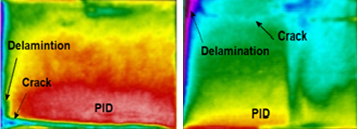
The most common faults that can found in PV plants in the site used for this study include delamination, cell crack, burn marks, potential induced degradation (PID), soiling effect, open string (Hot module), and junction box failure. IR images and I-V characteristics measured in the present study corresponding to each of the above faults are presented and discussed in Table 2. I-V measurements are used to calculate the module degradation factor (MDF) given by Eq. (1). The percentage (MDF) can be used for any types of affected modules at different times and different scales [36].
%MDF = (1-ISC (degraded) / ISC (Ideal) ×100 (1)
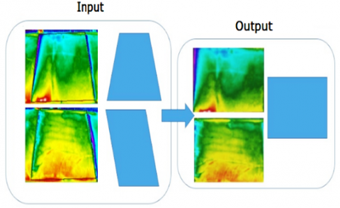
By using the IR camera, the images of modules are captured and image processing has been done. Image processing includes image filtering and panels reshape using pixel-shifting techniques. In our methodology, moving average filter and multidimensional filter are used. The geometric transformations are used to correct distortions caused by viewing geometry using pixel-shifting techniques to reshape that panel into a rectangular shape, as shown in Figure 1. The destination image is filled by regular scan lines, taking the values from the source image by bi-cubic interpolation. This has been done by applying geometric transformations to images. After getting the rectangular shape the cropping process can easily be done to remove unwanted segments. The next step is feature extraction methods. The feature extractions proposed in the present study are based on two types of feature extraction, namely, mathematical parameters-based feature extraction and on-line IV measurement-based feature extraction. The present adopted procedure for the fault detection and diagnosis using IRT and IV measurements is shown in Figure 2.
Figure 1. Reshaping and cropping of PV images
Figure 2. The present adopted procedure for the fault detection and diagnosis using IRT and IV measurements
4.1 Mathematical parameters-based feature extraction for thermal images
Our feature extraction depends on the mathematical relationships of temperature distributions and diffusions, which could be used for fault detection. These features deal with the temperature of thermal image or pixels, it includes the following:
Table 2. Failure cause and effect of CIGS thin-films
|
CIGS thin-film fault type |
Failure Cause |
Failure Effect |
|
|
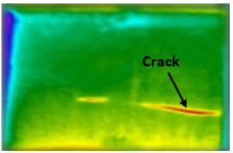
(a) Crack |
- The difference in thermal expansion and contraction of cell components. - Vibration during shipment (poor packaging). - Wind/snow load. |
- The shape and length of cell cracks affect the output of power and result in power loss causing a hot region. - The power can drop in beyond acceptable/warranty limits as it can reach to zero. - When the electrically isolated fragments do not transport charge carriers and therefore do not heat up, they stay cold. |
|
|
Cell crack causing a hot region |
|||
|
MDF = 46.15% |
|||
|
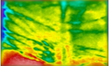
Cell cracks causing zero power output |
|||
|
I=0 V=0 |
|||
|
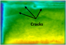
Cracks causing a cold area |
|||
|
MDF = 56.4% |
|||
|
(b) Junction box failure |
- Poor fixing of the junction box to the backsheet. - Due to poor manufacturing processes, j-boxes may open or badly closed. - Corrosion in both the connections and the string interconnects in the j-box due to Moisture. - Internal arcing in the j-box as a result of Bad wiring. |
- Arcing (inside junction box) - Ground fault - Corrosion Power drop beyond warranty limit due to a severe increase in series resistance |
|
|
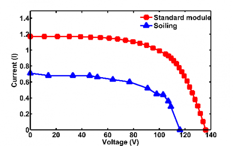
(c) Soiling |
- Low tilt angle of modules in locations exposed to pollution with irregular rainfall. - As a result of the lack of a bypass diode, the thin -films solar cells are subject to degradation due to the effects of shading. - Irregular cleaning of the surfaces of the modules. |
- The power loss where the max peak point is reduced. The Shadow effect may be soft or hard which affects the current and voltage of the PV module [37]. MDF = 39.32% |
|
|
CIGS thin-film fault type |
Failure Cause |
Failure Effect |
|
|
(b) Junction box failure |
- Poor fixing of the junction box to the backsheet. - Due to poor manufacturing processes, j-boxes may open or badly closed. - Corrosion in both the connections and the string interconnects in the j-box due to Moisture. - Internal arcing in the j-box as a result of Bad wiring. |
- Arcing (inside junction box) - Ground fault - Corrosion Power drop beyond warranty limit due to a severe increase in series resistance |
|
|
(d) Burn marks |
- Thermal expansion and contraction - No stress relief for interconnects - Use of non-softer ribbon - Poor quality of solder bonds (alloy/process) |
- Power drop beyond warranty limit due to severe series resistance. MDF = 64.95% |
|
|
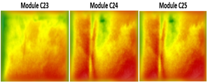
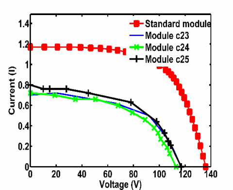
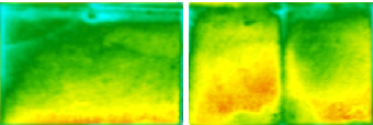
(e) PID |
- It occurs at high temperatures, in high humidity, and at high voltages approximately to the end of long strings |
- Significant degradation of the series resistance and therefore the power of the modules MDFC23= 40.17%, MDFC24=38.46%, MDFC25 = 31.62% |
|
|
(f) Open String |
- when the module string is not connected to the converter or the electric connection has lost the modules operating in the open circuit which means no electric energy is generated, as the energy converted to heat. |
- The electric power output is zero. |
|
4.1.1 Peak to peak value (PP)
It is a measure of the range of temperature variation overall the panel regardless of how this variation occurs. For the temperature of the thermal image of PV module, PP is equal to:
PP = Tmax – Tmin (2)
where, Tmax is the maximum pixel temperature, and Tminis the minimum pixel temperature.
4.1.2 Flatness density measure (FDM)
It is a measure of the flatness of portions having the peak value, in other words, it is the number of pixels having the peak value simplicity the peak points are considered to be within the range ≥0.95 of the peak value, Flatness measure [FM] is equal to:
$F D M=(( \sum \text {peak pixels} ) /( totlal number of pixels ))$ (3)
In Figure 3, the defective PV modules have different temperatures, the high temperature indicates the peak value, the thermal image consists of the number of pixels having different temperatures, the pixel that points to high temperature is called the peak, so each module has its specific FDM value.
Figure 3. PV modules with different flatness density measure
4.1.3 Flatness continuity measure (FCM)
It is defined as a measure of the maximum flatness of defect portion/s in PV module.
$F C M=\frac{\sum \text {peak pixels}}{\text {No of flat Portions}}$ (4)
In the case, if the defective modules have the same flatness density measure, the flatness continuity measure can distinguish between them and therefore detect the type of defects as shown in Figure 4.
Figure 4. PV difference between flatness density measure and flatness continuity measure
4.1.4 Global form factor (GFF)
It is defined using Eq. (5); to consider how the temperature of pixels varies and to measure the closeness of pixels temperature values to each other.
$G F F=\frac{N \times p e a k v a l u e}{\sum_{j=i}^{N l} \sum_{i=1}^{N w} T_{i, j}}$ (5)
where, N is the total number of pixels, Nw is the number of rows, Nl is the number of columns and Ti,j is the pixel temperature at (i, j).
4.1.5 Maximum form factor measure (FFmax)
In the maximum form factor, each column or row pixels are replaced by the maximum value for both horizontal and vertical views. It is defined as shown in Eq. (6, 7).
Maximum form factor in the width direction (vertical).
$F F_{\max v}=\frac{N_{l} \times \max \left\{\max _{j} T_{i, j}\right\}}{\sum_{i=1}^{N_{L}}\left\{\max _{j} T_{i, j}\right\}}$ (6)
Maximum form factor in the length direction (horizontal).
$F F_{\operatorname{maxh}}=\frac{N_{w} \times \max \left\{\max _{i}\left\{T_{i, j}\right\}\right\}}{\sum_{j=1}^{N_{w}}\left\{\max _{i} T_{i, j}\right\}}$ (7)
4.1.6 Mean form factor measure $\left(F F_{m n}\right)$
In the mean form factor, each row or column pixels are seen as a single pixel, having their mean value. Then the form factor is calculated from the resultant mean values for both horizontal and vertical views. It is clear that the mean form factor is less than the maximum form factor since the max value is greater than or equal to the mean value. It is defined in Eq. (8, 9).
The mean form factor in the width direction (vertical).
$F F_{m n v}=\frac{N_{l} \times \max \left\{\sum_{i=1}^{N_{w}} T_{i, j}\right\}}{N_{w} \times \sum_{j=1}^{N_{i}} \sum_{i=1}^{N_{w}} T_{i, j}}$ (8)
The mean form factor in the length direction (horizontal).
$F F_{m n h}=\frac{N_{w} \times \max \left\{\sum_{j=1}^{N_{l}} T_{i, j}\right\}}{N_{l} \times \sum_{i=1}^{N_{w}} \sum_{j=1}^{N_{l}} T_{i, j}}$ (9)
4.1.7 The 1st order zero temperature change rate (ω)
It is related to; how many pixels are zero and their temperature < peak value. It’s a measure of how heat diffusion and extended. It is defined by the following equations.
$\begin{aligned} d T V_{i, k} &=T_{i, k+1}-T_{i, k} \\ \forall 1 & \leq k \leq N_{l-1} \\ 1 & \leq i \leq N_{w} \end{aligned}$ (10)
where, $d T V$ is the first order derivative of temperature in vertical direction and K is the column order.
$d T H_{Z, j}=T_{Z+1, j}-T_{Z, J} \\ \forall 1 \leq Z \leq N_{W-1} \\ 1 \leq Z \leq N_{l}$ (11)
where, $d T H$ is the first order derivative of temperature in the horizontal direction and Z is the row order.
Then
$\omega_{v}=\frac{\text {No.of }\{d T V<\varepsilon\}}{N}$ (12)
$\omega_{h}=\frac{\text {No.of }\{D T H<\varepsilon\}}{N}$ (13)
where, $\omega_{v}$ is the 1st order zero temperature change rate in the vertical direction, ɛ is the very low value ≈.01 and $\omega_{h}$ is the 1st order zero temperature change rate in the horizontal direction.
4.1.8 The 2nd order zero temperature change rate (ώ)
It is considered for the second change rate of temperature also, it’s a measure of how heat diffusion and extended. It is defined in the following equations.
$d 2 T V_{i, k}=d T V_{i, k+1}-d T V_{i,} \\ \forall 1 \leq K \leq N_{l-1} \\ 1 \leq k \leq N_{w}$ (14)
here $d 2 T V$ is the second order derivative of temperature in the vertical direction and K is the column order.
$d 2 T H_{Z, J}=d T H_{Z+1, i}-d T H_{Z, i} \\ \forall 1 \leq Z \leq N_{w-1} \\ 1 \leq j \leq N_{L}$ (15)
where, $d 2 T H$ is the second order derivatives of temperature in the horizontal direction.
Then
$\bar{\omega}_{V}=\frac{\text {No. of }\{d 2 T V<\varepsilon\}}{N}$ (16)
$\bar{\omega}_{h}=\frac{\text {No.of }\{d 2 T H<\varepsilon\}}{N}$ (17)
where, $\bar{\omega}_{V}$ is the 2nd order zero temperature change rate the vertical direction and $\bar{\omega}_{h}$ is the 2nd order zero temperature change rate in the horizontal direction.
4.1.9 Cold area percentage measure (CPM)
Faults like delamination and cracks (in some cases) may cause cold area (inactive area) within PV module, this measure determines the percentage of the cold area if appear within the module. The inactive area makes a shortage in current and voltage and consequently in power output. For a high percentage of cold areas, the cell considers being dead cell and the cell should be replaced. The cold points are considered to be within the range ≤0.5 of the cold value, it is defined as shown in Eq. (18)
$\mathrm{CPM}=(( \sum \text {coldpixels} ) / (totlal number of pixels)) $ (18)
4.1.10 percentage factor measure (PFM)
The module is divided into some divisions based on a selected percentage (10%) from the bottom of modules, and for each division, the above feature extractions are calculated, it can measure the variation of these features within modules, it can detect many types of faults within modules. For example, the use of percentage factor measure with global form factor (PGFF), mean calculate the GFF at each division. The symbol of percentage factor measure changes with the type of selected feature, e.g. the percentage factor measure by using the maximum form factor for horizontal is denoted as $\left(P F F_{\operatorname{maxh}}\right)$ where the letter P is written before the symbol of feature and so on.
4.2 On line I-V measurements-based feature extraction
Since the thermal imaging is carried out during normal operation of the PV modules, the features based on electrical measurements are restricted by the operating voltage, current, and power. The features are calculated by comparing the operating value to its corresponding healthy one for operating voltage, current, and power (Ir, Vr, and Pr) also, efficiency and fill factor are calculated [38] where,
Operating current ratio
Ir = Io / Ih (19)
Operating voltage ratio
Vr = Vo / Vh (20)
Operating power ratio
Pr = Po / Ph (21)
Fill factor
FF = Io × Vo / Isc × Voc (22)
Efficiency
Ƞ= Isc × Voc × FF / Pin × A (23)
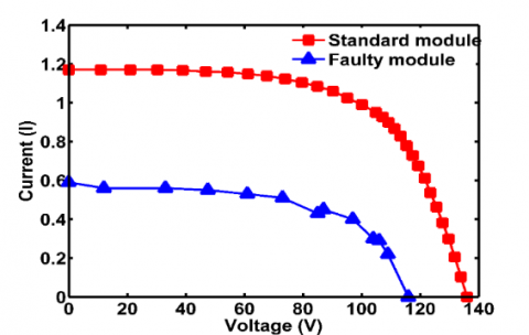
where, Io, Vo, and Po are the operating current, voltage, and power of the inspected module respectively, Ih, Vh, and Ph are the maximum operating current, voltage, and power of the healthy module respectively, FF is the fill factor, Isc is the short circuit current, Vocis the open circuit voltage, Pin is the input power for efficiency calculations is 1 kW/m2 or 100 mW/cm2 and A is the cell area (cm2). As the healthy values for the electric parameters vary with time depending on the solar irradiation and electrical load, they could be considered as the maximum operating voltage, current, and power of all on-operations PV modules. Figure 5 represents I-V curves of the defective PV module and the standard one and its influence on the maximum power. For all faults, Ir, Vr, Pr, efficiency and fill factor are evaluated.
Figure 5. I-V curves of the standard module and faulty module (module d11)
The datasets are generated by utilizing the thermal images and IV measurements of inspected modules; also, the mathematical parameters-based feature extraction is obtained by using the MATLAB platform. For this study most of the modules have more than one fault, the faults are categorized as illustrated in Table 3.
A general classification matrix of CIGS faults using features of mathematical parameters techniques and IV measurements is shown in Table 4. It defines the features required for distinguishing among different faults. The first row and column of the matrix indicate the fault type. The inner rows and columns contain the electrical measurements and the mathematical parameters-based features extraction that can be used to distinguish between faults. Taking for example fault type A, the features that can distinguish between fault type A and fault type B are peak to peak (PP), 1st order zero temperature change rate (ω), electrical measurements (EM), and maximum form factor for horizontal $F F_{\operatorname{maxh}}$), and so on for the whole of the table. In the case where the fault type contains more than one fault, the percentage of some features such as ($F F_{\operatorname{maxh}} / F F_{\max v}$) and ($F F_{m n h} / F F_{m n v}$) can help in the detection of this type of faults such as in the case of fault of type B and type C. Also, the percentage factor measure using the mean form factor for horizontal ($P F F_{m n h}$) and vertical ($P F F_{m n v}$) and the percentage factor measure using maximum form factor for horizontal ($\left.P F F_{\operatorname{maxh}}\right)$) and vertical ($P F F_{\operatorname{maxv}}$) are used in distinguishing between these types of faults.
Table 3. Faults categories
|
Type A |
Soiling |
|
Type B |
Soiling and crack |
|
Type C |
Burn marks, soiling, and crack |
|
Type D |
Potential induced degradation (PID) |
|
Type E |
PID and crack |
|
Type F |
PID, crack, and delamination |
|
Type G |
Open string (HM) |
|
Type H |
Dead module |
Table 4. General failures classification matrix of CIGS thin-film module using features based on mathematical parameters and electrical measurements
|
Fault Type |
A |
B |
C |
D |
E |
F |
G |
H |
|
A |
|
ω EM pp $F F_{maxh}$ $F F_{maxg}$/ $F F_{maxv}$ |
GFF EM pp $F F_{m n h}$ |
$F F_{m n v}$ GFF PGFF $F F_{maxh}$
|
$F F_{m n v}$ $F F_{m a x h}$ GFF |
$F F_{m a x h}$ $F F_{m n h}$ $F F_{m a x v}$ GFF |
CPM $F F_{m a x h}$ $F F_{m a x v}$ $F F_{m n h}$ $F F_{m n v}$ GFF FDM FCM |
EM PP ( $F F_{m a x h}$/ $F F_{m a x v}$ ) ( $F F_{m n h}$ / $F F_{m n v}$ )
|
|
B |
|
|
EM $\left(F F_{\operatorname{maxh}} / F F_{\max v}\right)$ $P F F_{\operatorname{maxh}}$
|
GFF EM PGFF |
GFF |
$F F_{m n h}$ EM
|
CPM $F F_{m n v}$ GFF $P F F_{m n h}$ FDM FCM |
EM GFF $F F_{\text {maxh}}$ |
|
C |
|
|
` |
$F F_{m n h}$ GFF EM
|
$F F_{m n h}$ GFF EM
|
$F F_{\operatorname{maxh}}$ GFF $F F_{\operatorname{maxh}}$
|
CPM $F F_{\operatorname{maxh}}$ GFF FDM |
($\left(F F_{\operatorname{maxh}} / F F_{\max v}\right)$ EM
|
|
D |
|
|
|
|
CPM GFF $F F_{m n h}$
|
PP EM
|
CPM $F F_{m n v}$ GFF |
EM FDM PP $F F_{m n h}$ |
|
E |
|
|
|
|
|
$\left(F F_{\operatorname{maxh}} / F F_{\operatorname{maxv}}\right)$
|
CPM $F F_{m n h}$ GFF ω |
EM $F F_{m n h}$ GFF PP |
|
F |
|
|
|
|
|
|
CPM $F F_{m n v}$ GFF ω |
EM $F F_{m n h}$ |
|
G |
|
|
|
|
|
|
|
$F F_{m n h}$ FDM GFF EM CPM |
Table 5. Failure modes analysis and diagnostic architecture for CIGS thin-film PV
|
Features Faults |
PP |
FDM |
FCM |
$F F_{\operatorname{maxh}}$ |
$F F_{\operatorname{maxv}}$ |
$F F_{\operatorname{mnh}}$ |
$F F_{\operatorname{mnv}}$ |
GFF |
$\omega_{h}$ |
ώh |
CP |
|
Type A (module a7) |
146 |
0.1168 |
12872 |
0.6859 |
0.9148 |
0.6859 |
0.8221 |
0.5880 |
0.7403 |
0.8094 |
0.1031 |
|
Type B (module d22) |
145 |
0.2034 |
1282 |
0.8878 |
0.9453 |
0.8234 |
0.8544 |
0.7667 |
0.8645 |
0.7964 |
0.0042 |
|
Type C (module d21) |
176 |
0.0096 |
1729 |
0.8029 |
0.8832 |
0.6568 |
0.8182 |
0.5712 |
0.8774 |
0.9315 |
0.0007 |
|
Type D (module b4) |
176 |
0.0002 |
26 |
0.8147 |
0.8302 |
0.9715 |
0.9349 |
0.7362 |
0.8809 |
0.9326 |
0.0027 |
|
Type E (module c5) |
146 |
0.1264 |
15313 |
0.9340 |
0.9225 |
0.9047 |
0.9225 |
0.8150 |
0.8503 |
0.9230 |
0.0088 |
|
Type F (module b18) |
151 |
0.0309 |
3704 |
0.9017 |
0.9189 |
0.91111 |
0.9395 |
0.8497 |
0.9026 |
0.8023 |
0.0170 |
|
Type G (module a23) |
142 |
0.4140 |
47706 |
0.9672 |
0.9679 |
0.9378 |
0.9679 |
0.9545 |
0.7599 |
0.7599 |
0 |
|
Type H (module a25) |
126 |
0.3567 |
42138 |
0.9505 |
0.9599 |
0.9143 |
0.9335 |
0.9313 |
0.9238 |
0.9489 |
0 |
Table 6. The mean and standard deviation of mathematical parameters-based features extraction of CIGS thin-film PV module
|
Features Faults |
PP |
FDM |
FCM |
$F F_{\operatorname{maxh}}$ |
$F F_{\operatorname{maxv}}$ |
|||||
|
Mean |
ST. D |
Mean |
ST. D |
Mean |
ST. D |
Mean |
ST. D |
Mean |
ST. D |
|
|
Type A |
145.33 |
13.064 |
0.0715 |
0.0482 |
7860 |
5342.6 |
0.7269 |
0.1002 |
0.8826 |
0.0645 |
|
Type B |
170.55 |
23.964 |
0.0459 |
0.0615 |
3501.6 |
4409.8 |
0.8022 |
0.1545 |
0.8879 |
0.0927 |
|
Type C |
163.5 |
10.5987 |
0.0546 |
0.0749 |
2170 |
441.4 |
0.7114 |
0.1303 |
0.9099 |
0.0297 |
|
Type D |
155 |
20.15 |
0.188 |
0.1485 |
22236 |
17691 |
0.9228 |
0.0595 |
0.9233 |
0.071 |
|
Type E |
156.625 |
16.4572 |
0.0938 |
0.0917 |
11110 |
10886 |
0.876 |
0.0721 |
0.9249 |
0.0449 |
|
Type F |
177.5 |
32.9596 |
0.0706 |
0.1166 |
8426.8 |
13900 |
0.96 |
0.0464 |
0.8306 |
0.1326 |
|
Type G |
146 |
9.798 |
0.2249 |
0.0951 |
26688 |
11715 |
0.9428 |
0.0155 |
0.9536 |
0.01 |
|
Type H |
161.77 |
25.37 |
0.0718 |
0.0954 |
8554 |
11326 |
0.8658 |
0.142 |
0.8929 |
0.0895 |
|
Features Faults |
$F F_{m n h}$ |
$F F_{m n v}$ |
GFF |
$\omega_{h}$ |
ώh |
CP |
|||||||
|
Mean |
ST. D |
Mean |
ST. D |
Mean |
ST. D |
Mean |
ST. D |
Mean |
ST. D |
Mean |
ST. D |
||
|
Type A |
0.6445 |
0.1578 |
0.7876 |
0.0799 |
0.5295 |
0.0503 |
0.8253 |
0.0717 |
0.8461 |
0.0738 |
0.0483 |
0.0489 |
|
|
Type B |
0.6275 |
0.117 |
0.7536 |
0.1599 |
0.5626 |
0.1479 |
0.8677 |
0.0395 |
0.8478 |
0.0652 |
0.0437 |
0.071 |
|
|
Type C |
0.6242 |
0.1158 |
0.8638 |
0.0385 |
0.5769 |
0.1141 |
0.8879 |
0.0097 |
0.8295 |
0.0682 |
0.0417 |
0.0442 |
|
|
Type D |
0.8598 |
0.1442 |
0.8612 |
0.1537 |
0.8043 |
0.161 |
0.882 |
0.0405 |
0.8775 |
0.081 |
0.0247 |
0.0861 |
|
|
Type E |
0.8176 |
0.128 |
0.8619 |
0.1047 |
0.7619 |
0.1236 |
0.8686 |
0.0267 |
0.8961 |
0.0602 |
0.0183 |
0.0278 |
|
|
Type F |
0.8139 |
0.2232 |
0.7137 |
0.3052 |
0.6757 |
0.2697 |
0.8734 |
0.0283 |
0.8588 |
0.0782 |
0.0934 |
0.1744 |
|
|
Type G |
0.9308 |
0.0215 |
0.9598 |
0.0069 |
0.9186 |
0.0212 |
0.899 |
0.051 |
0.8467 |
0.0659 |
0 |
0 |
|
|
Type H |
0.7804 |
0.1869 |
0.8169 |
0.1766 |
0.6981 |
0.2132 |
0.8733 |
0.044 |
0.897 |
0.0585 |
0.0231 |
0.0602 |
|
During the study, it was observed that the values of the first order zero temperature change rate ω, in the case of horizontal and vertical are almost equal, so only the horizontal was used and takes symbol $\omega_{h}$. The same case is in the second zero temperature change rate, the horizontal is used and takes symbol (ώh). The vertical is dispensed with to avoid duplicating data that will have little value.
5.1 Analysis of mathematical parameters-based features extraction
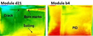
To explain how the mathematical Parameters-based feature can distinguish between faults, this can be illustrated in Table 5. Where it shows the values of mathematical parameters obtained from IR image analysis of CIGS PV modules with different faults. The process of distinguishing between faults is done by comparing the values of features of the faults. For further clarification, the fault of module a7 belongs to type A, and the fault of module c5 belongs to type E. It can be noticed that the peak to peak measure (PP) of the two modules has the same value, but features such as maximum form factor measure for the horizontal ($F F_{\operatorname{maxh}}$) , means form factor for the horizontal ($F F_{\operatorname{mnh}}$), global form factor (GFF), and some other features can distinguish between them. The interpretation of these values of the features is explained in Figure 6. The same steps are done for module d21 (fault type C) and module b4 (fault type D), where the values of the peak to peak measure (PP) of the two type of faults are the same, where the features flatness density measure (FDM), flatness continuity measure (FCM) and global form factor (GFF) can distinguish between them as shown in Figure 7. The same steps are implemented between all types of faults to extract the features that can distinguish between faults.
The temperature distribution analysis of different technologies of PV modules using infrared thermography has been discussed by Gulkowski et al. [34]. Due to the difference in IR technology, each technology has been shown to have a specific temperature range for different faults. The main advantage of using the present proposed mathematical parameters is that it doesn't depend on the temperature variation and it is applicable for any technology of PV.
The data set is classified into each type of fault as represented in Table 3. The mean and standard deviation for each type of fault, based on the mathematical parameters, are illustrated in Table 6. The standard deviations of some features are large and that of other features is low. For example, for fault type F, the feature peak to peak (PP) has a high mean and standard deviation values. To explain the reason, Figure 8 shows two modules of type F, the hot region of module b18 is more than in module b7 and there is variation in temperature which results in a high standard deviation. Also, Figure 9 indicates the reason that the mean and standard deviation of feature flatness continuity measure (FDM) for fault type B is low. The fault of type G has high mean values for the features, flatness density measure (0.2249), flatness continuity measure (26688), maximum form factor measure for the vertical (0.9536), mean form factor measure for the horizontal and vertical respectively (0.9308, 0.9598), and The 1st order zero temperature change rate (0.899) and the standard deviations of this type of faults are small. The fault of type G represents the hot modules (open string), as shown in Table 2(f), which mean that most of the cell is hot, the values of this features show that it has the ability of identification as its values are high, while the Cold area percentages measure should be equal to zero.
Figure 6. IR images of faulty modules represent type A (module a7) and type E (module a5)
Figure 7. IR images of faulty modules represent type C (module d21) and type D (module b4)
Figure 8. The hot region of two faulty modules of type F
Figure 9. Two modules represent the fault of type B
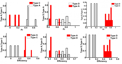
Peak to peak measure (PP), the flatness density measure (FDM), the flatness continuity measure (FCM), and the global form factor (GFF) for the fault of type D is higher than the fault of type A as shown in Table 6. The fault of type D is related to PID. When the module is subjected to PID, part of the modules, or may all the module be hot, the temperature of modules subjected to PID is higher than that subjected to soiling as in the case of type A. For more identification, a histogram for some of the suggested features between types A and D is illustrated in Figure 10 (a), the Figures indicate the features that can distinguish between the type A and D and the overlap features.
Figure 10. Histograms of some faults to indicate the effect of features in the classification (a) histogram between fault type A and D, (b) histogram between fault type A and B, (c) histogram between fault type B and E and (d) histogram between fault type A and C
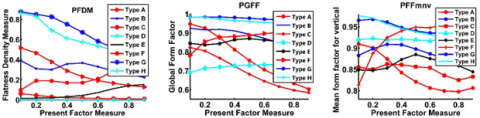
Figure 11. Percentage factor measure using (a) flatness density measure (PFDM), (b) global form factor (PGFF) and (c) mean form factor for vertical (
Figure 12. Histograms of power output and efficiency to indicate the fault classification
Histograms of some faults can indicate the effect of features in the classification as shown in Figure 10. In the case of type, A and type B faults, the percentage of maximum form factor for horizontal to maximum form factor for vertical $\left(F F_{\operatorname{maxh}} / F F_{\max v}\right)$ has effect value in the classification. The most effective feature that can distinguish between type B and type E is the Global form factor feature. Also, some features that effect in classification between type A and C is illustrated.
The percentage factor measure (PFM) is implemented as the following; first detect the type of feature which required to measure, second for each type of fault, select the modules. Table 5 shows each module belongs to its fault; these modules are examined by using the percentage factor measure. Some features such as flatness density measure (FDM), global form factor (GFF), and mean form factor for vertical $\left(\mathrm{FF}_{\mathrm{mnv}}\right)$ are selected to calculate percentage factor measure (PFM) as illustrated in Figure 11. The name of these features will be (PFDM), (PGFF) and ($\left(\mathrm{P} F F_{m n v}\right)$), where the symbol P refers to the percentage factor measure. Figure 11(a) represents flatness density measure using percentage factor measure $(P G F F)$ for selected modules, it shows there is variation between all modules except the modules related to the fault of type C and fault of type H. For feature (PGFF ) in Figure 11(b) shows the variation between faults except the modules related to the fault of type G and fault of type H, and so on as for Figure 11(c). The percent factor measure shows its capability to distinguish between faults.
5.2 Analysis of online I-V measurements-based feature extraction
The electrical measurements (EM) include a current operating ratio (Ir), voltage operating ratio (Vr), power operating ratio (Pr), efficiency (Ƞ), and fill factor (FF). The type of fault and its area affect the production of power and, consequently, the efficiency, and the fill factor. The histogram of Power ratio and efficiency of CIGS faults are shown in Figure 12(a). The power ratio output can distinguish between faults of type A and C and also between faults of type C and D, but it can't distinguish between the type of faults A and D, the same in the case of efficiency in Figure 12(b). The classification between faults using the electrical measurements is shown in the general classification matrix in Table 4.
This work presents a novel technique for faults diagnosis of CIGS PV modules by extracting features based on mathematical parameters of thermal images and electrical measurements. Common faults of CIGS thin-film PV modules are classified and corresponding I-V measurements and IRT images are obtained in outdoor conditions following standard guidelines. The proposed mathematical parameters-based features are extracted from 2D matrix of the thermal image. The capability and robustness of the new proposed methodology to distinguish between different fault types and defective modules with more than one fault type is demonstrated. This capability is very essential for maintenance planning in identifying and avoiding occurrence and determining the proper maintenance action. Previous studies were limited by the detection hotspots or defective modules regardless of the fault type.
The global form factor feature (GFF) is found to be the most effective feature in the diagnosis process as it measures the temperature variation of pixels based on the type of fault. The module temperature is a function of fault type and gradually increases from relatively low values for soiled modules, moderate values for PID, and high values for the hot modules. For soiled modules, the existence of additional faults increases the average value of (GFF). Accuracy in dealing with the detection of faults is improved by analyzing the maximum and mean variation of temperature in both the horizontal and vertical directions. The proposed features do not deal directly with pixel temperatures or pixel values and are therefore shown to be independent of variation in temperature that may result from the use of different infrared cameras sensors. Also, they can describe the shape of faults patterns for cold and hot areas. A general classification matrix is established that summarizes the correlations between fault type and associated features. This matrix is very useful for maintenance planning and automation.
|
2D |
2 dimensional |
|
A |
the cell area (cm2) |
|
CdTe |
cadmium telluride |
|
CIGS |
copper Indium Gallium Selenide |
|
CPM |
cold area percentages measure |
|
c-Si |
crystalline silicon |
|
$d T H$ |
first order derivatives of temperature in horizontal direction |
|
$d T V$ |
first order derivatives of temperature in vertical direction |
|
E |
solar irradiance |
|
$F F_{\operatorname{maxh}}$ |
maximum form factor for horizontal |
|
$F F_{\operatorname{maxv}}$ |
maximum form factor for vertical |
|
$F F_{\operatorname{mnh}}$ |
mean form factor for horizontal |
|
$F F_{\operatorname{mnv}}$ |
mean form factor for vertical |
|
$T_{i, j}$ |
represents pixel temperature at (i, j). |
|
FCM |
flatness continuity measure |
|
FDD |
fault detection and diagnosis |
|
FDM |
flatness density measure |
|
FF |
Fill factor |
|
GFF |
global form factor |
|
GW |
Gigawatts |
|
I |
Current |
|
Ih |
maximum operating current of the healthy module |
|
Io |
operating current of the inspected module |
|
Ir |
operating current ratio |
|
IRT |
infrared thermography |
|
Isc |
short circuit current |
|
IV |
current- voltage measurements |
|
K |
column order |
|
MDF |
module degradation factor |
|
N |
total number of pixels |
|
Nl |
the number of columns |
|
NNs |
Neural networks |
|
Nw |
the number of rows |
|
P |
power output |
|
$P F F_{\operatorname{maxh}}$ |
percentage factor measure using the maximum form factor for horizontal |
|
$P F F_{\operatorname{mnv}}$ |
percentage factor measure using the mean form factor for vertical. |
|
pc-Si |
polycrystalline silicon |
|
PFDM |
percentage factor measure using flatness density measure |
|
PFM |
Percentage factor measure |
|
PGFF |
Percentage factor measure using the global form factor |
|
Ph |
maximum operating power of a healthy module |
|
PID |
potential induced degradation |
|
Pin |
1 kW/m2 or 100 mW/cm2 |
|
Pmax |
maximum power output of standard module (w) |
|
Po |
operating power of an inspected module |
|
PP |
peak to peak |
|
Pr |
operating power ratio |
|
PV |
photovoltaic |
|
PVM |
photovoltaic module |
|
ROI |
region of interest |
|
Tamb |
ambient temperature |
|
TFE |
texture feature extraction |
|
Tmax |
maximum pixel temperature |
|
Tmin |
minimum pixel temperature |
|
UV |
ultraviolet |
|
V |
voltage |
|
Vh |
maximum operating voltage of the healthy module |
|
Vo |
operating voltage of the inspected module |
|
Voc |
open circuit voltage |
|
Vr |
operating voltage ratio |
|
Z |
row order |
|
Greek symbols |
|
|
ɛ |
the very low value ≈.01 |
|
Ƞ |
Efficiency |
|
ω |
the 1st order zero temperature change rate |
|
ώ |
the 2nd order zero temperature change rate |
|
ωh |
the 1st order zero temperature change rate in horizontal direction |
|
ώh |
the 2nd order zero temperature change rate in horizontal direction |
|
ωv |
the 1st order zero temperature change rate in vertical direction |
|
ώv |
the 2nd order zero temperature change rate in vertical direction |
|
Ω |
Ohm |
[1] Thin-Film Photovoltaic (PV) Cells Market Analysis to 2020 - CIGS (Copper Indium Gallium Diselenide) to Emerge as the Major Technology by 2020. GBI Research, 1-4.
[2] Buerhop, C., Jahn, U., Hoyer, U., Lerche, B., Wittmann, S. (2007). Final report of the feasibility study to check the quality of photovoltaic modules by means of infrared recording. Technical Report. Bayern, Erlangen.
[3] Moropoulou, A., Palyvos, J., Karoglou, M., Panagopoulos, V. (2007). Using IR thermography for photovoltaic array performance assessment. Proc. 4th International Conference on NDT - Hellenic Society for NDT, pp. 1804-1806.
[4] Zefri, Y., ElKettani, A., Sebari, I., Lamallam, S. (2018). Thermal Infrared and visual inspection of photovoltaic installations by UAV photogrammetry—application case: Morocco. Drones, 2(4): 41. https://doi.org/10.3390/drones2040041
[5] Prakash, R. (2019). Infrared Thermography. InTech, p. 222. https://doi.org/10.5772/1353
[6] Irshad, Jaffery, Z.A., Haque, A. (2018). Temperature measurement of solar module in outdoor operating conditions using thermal imaging. Infrared Physics & Technology, 92: 134-138. https://doi.org/10.1016/j.infrared.2018.05.017
[7] Buerhop, C., Pickel, T., Scheuerpfluga, H., Camusa, C., Haucha, J., Brabec, C.J. (2016). Statistical overview of findings by IR-inspections of PV-plants. Proceedings Volume 9938, Reliability of Photovoltaic Cells, Modules, Components, and Systems IX; 99380L. https://doi.org/10.1117/12.2237821
[8] Buerhop-Lutz, C., Scheuerpflug, H., Pickel, T. (2015). Defect analysis of installed PV-modules-IR-thermography and in-string power measurement. European Photovoltaic Solar Energy Conference and Exhibition, pp. 1692-1697. https://doi.org/10.4229/EUPVSEC20152015-5BO.12.6
[9] Zefri, Y., Elkcttani, A., Sebari, I., Lamallam, S.A. (2017). Inspection of photovoltaic installations by thermo-visual UAV imagery application case: Morocco. International Renewable and Sustainable Energy Conference (IRSEC), Tangier, pp. 1-6. https://doi.org/10.1109/IRSEC.2017.8477241
[10] Takyi, G. (2017). Correlation of infrared thermal imaging results with visual inspection and current-voltage data of PV modules installed in Kumasi, a Hot, Humid Region of Sub-Saharan Africa. Technologies, 5(4): 67. https://doi.org/10.3390/technologies5040067
[11] Hu, Y., Cao, W., Ma, J., Finney, S.J., Li, D. (2014). Identifying PV module mismatch faults by a thermography-based temperature distribution analysis. IEEE Transactions on Device and Materials Reliability, 14(4): 951-960. https://doi.org/10.1109/TDMR.2014.2348195
[12] Tsanakas, J.A., Ha, L., Buerhop, C. (2016). Faults and infrared thermographic diagnosis in operating c-Si photovoltaic modules: A review of research and future challenges. Renewable and Sustainable Energy Reviews, 62: 695-709. https://doi.org/10.1016/j.rser.2016.04.079
[13] Buerhop, C.I., Schlegel, D., Niess, M., Vodermayer, C., Weißmann, R., Brabec, C.J. (2012). Reliability of IR-imaging of PV-plants under operating conditions. Solar Energy Materials and Solar Cells, 107: 154-164. https://doi.org/10.1016/j.solmat.2012.07.011
[14] Buerhop-Lutz, C., Scheuerpflug, H., Pickel, T. (2015). Defect analysis of installed PV-modules – IR-thermography ad in-string power measurement. 31st European Photovoltaic Solar Energy Conference and Exhibition, pp. 1692-1697. https://doi.org/10.4229/EUPVSEC20152015-5BO.12.6
[15] Ebner, R., Zamini, S., Újvári, G. (2010). Defect analysis in different photovoltaic modules using Electroluminescence (EL) and Infrared (IR) Thermography. 25th European Photovoltaic Solar Energy Conference and Exhibition / 5th World Conference on Photovoltaic Energy Conversion, 6-10 September 2010, Valencia, Spain, pp. 333-336. https://doi.org/10.4229/25thEUPVSEC2010-1DV.2.8
[16] Roumpakias, E., Bouroutzikas, F., Stamatelos, A. (2016). On-site inspection of PV panels, aided by infrared thermography. Advances in Applied Sciences, 1(3): 53-62. https://doi.org/10.11648/j.aas.20160103.12
[17] Sahoo, P.K., Soltani, S., Wong, A.K.C. (1988). A survey of thresholding techniques. Computer Vision, Graphics, and Image Processing, 41(2): 233-260. https://doi.org/10.1016/0734-189X(88)90022-9
[18] Otsu, N. (1975). A threshold selection method from gray-level histograms. IEEE Transactions on Systems, Man, and Cybernetics, 9(1): 62-66. https://doi.org/10.1109/TSMC.1979.4310076
[19] Minor, L.G., Sklansky, J. (1981). The detection and segmentation of blobs in infrared images. IEEE Transactions on Systems, Man, and Cybernetics, 11(3): 194-201. https://doi.org/10.1109/TSMC.1981.4308652
[20] Maldague, X., Krapez, J.C., Poussart, D. (1990). Thermographic nondestructive evaluation (NDE): An algorithm for automatic defect extraction in infrared images. IEEE Transactions on Systems, Man and Cybernetics, 20(3): 722-725. https://doi.org/10.1109/21.57287
[21] Tsanakas, J.A., Botsaris, P. N. (2013). On the detection of hot spots in operating photovoltaic arrays through thermal image analysis and a simulation model. Materials Evaluation, 71(4): 457-465.
[22] Tsanakas, J.A., Botsaris, P.N. (2011). Passive and active thermographic assessment as a tool for condition-based performance monitoring of photovoltaic modules. J. Sol. Energy Eng., 133(2): 021012. https://doi.org/10.1115/1.4003731
[23] Ibarra-Castanedo, C., Gonzalez, D., Klein, M., Pilla, M., Vallerand, S., Maldague S.V.X. (2004). Infrared image processing and data analysis. Infrared Physics & Technology, 46(1-2): 75-83. https://doi.org/10.1016/j.infrared.2004.03.011
[24] Leotta, G., Pugliatti, P.M., Di Stefano, A., Aleo, F., Bizzarri, F. (2015). Post-processing technique for thermo-graphic images provided by drone inspections. In: Proceedings of the 31st European photovoltaic solar energy conference and exhibition (EU PVSEC). Hamburg, Germany, pp. 1799-1803. https://doi.org/10.4229/EUPVSEC20152015-5CO.15.5
[25] Rasch, R., Hantelmann, S., Dreimann, R., Behrens, G., Hamelmann, F.U., Weicht, J.A. (2015). Automated thermal imaging for fault detection on PV-systems. In: Proceedings of the 31st European photovoltaic solar energy conference and exhibition (EU PVSEC). Hamburg, Germany, pp. 2147-2149. https://doi.org/10.4229/EUPVSEC20152015-5BV.1.53
[26] Maldague, X.P. (2001). Getting started with thermography for nondestructive testing. Theory and Practice of Infrared Technology for Nondestructive Testing. Wiley-Interscience.
[27] Vollmer, M., Möllmann, K.P. (2010). Advanced Methods in IR Imaging. Infrared Thermal Imaging: Fundamentals, Research, and Applications. Weinheim: Wiley-VCH Verlag, 229-349.
[28] Hardy, G. (1997). Thermal Inspection. ASM Handbook – nondestructive evaluation and quality control. ASM International.
[29] Niazi, K., Akhtar, W., Khan, H.A., Sohaib, S., Nasir, A.K. (2018). Binary classification of defective solar PV modules using thermography. 2018 IEEE 7th World Conference on Photovoltaic Energy Conversion (WCPEC) (A Joint Conference of 45th IEEE PVSC, 28th PVSEC & 34th EU PVSEC), Waikoloa Village, HI, pp. 0753-0757. https://doi.org/10.1109/PVSC.2018.8548138
[30] Kurukuru, B., Haque, A., Kha, A., Tripathy, A.K. (2019). Fault classification for photovoltaic modules using thermography and machine learning techniques. International Conference on Computer and Information Science (ICCIS), pp. 1-6. https://doi.org/10.1109/ICCISci.2019.8716442
[31] Tsanakas, J.A., Chrysostomou, D., Botsaris, P.N., Gasteratos, A. (2015). Fault diagnosis of photovoltaic modules through image processing and canny edge detection on field thermographic measurements. International Journal of Sustainable Energy, 34(6): 351-372. https://doi.org/10.1080/14786451.2013.826223
[32] Buerhop, C., Fecher, F.W., Pickel, T., Häring, A., Adamski, T., Camus, C., Hauch, J., Brabec, C.J. (2018). Verifying defective PV‐modules by IR‐imaging and controlling with module optimizers. Special Issue: Key Papers from EU PVSEC 2017, 26(8): 622-630. https://doi.org/10.1002/pip.2985
[33] Buerhop, C., Pickel, T., Scheuerpflug, H., Dürschner, C. Camus, C., Hauch, J., Brabec, C. (2018). Verifying defective PV‐modules by IR‐imaging and controlling with module optimizers. Special Issue: Key Papers from EU PVSEC 2017, 26(8): 622-630. https://doi.org/10.1002/pip.2985
[34] Gulkowski, S., Zytkowska, N., Dragan, P. (2018). Temperature distribution analysis of different technologies of PV modules using infrared thermography. E3S Web of Conferences. https://doi.org/10.1051/e3sconf/20184900044
[35] Demirtaş, M., Tamyürek, B., Kurt, E., Çetinbaş, İ., Öztürk, M.K. (2019). Effects of aging and environmental factors on performance of CdTe and CIS thin-film photovoltaic modules. Journal of Electronic Materials, 48(11): 6890-900. https://doi.org/10.1007/s11664-019-07172-z
[36] Mohammad, R., Hashim, H., Chandima G., Mohd Amran R., Mohammad I., Shahrooz H. (2016). Power loss due to soiling on a solar panel: A review. Renewable and Sustainable Energy Reviews, 59: 1307-1316. https://doi.org/10.1016/j.rser.2016.01.044
[37] Grid connected photovoltaic systems – Minimum requirements for system documentation, commissioning tests, and inspection. (2009). IEC: Geneva, Switzerland.
[38] Ushasree P.M., Bora, B. (2019). Chapter 1: Silicon Solar Cells, in Solar Energy Capture Materials, pp. 1-55. https://doi.org/10.1039/9781788013512-00001