Maamar Latroch* | Derouazin Ahmed | Omari Abdelhafid
OPEN ACCESS
This paper is concerned with the sensor fault detection in mini UAVs quadrotor. We propose a detection algorithm based on the behavior of the Extended Kalman Gain Norm (EKGN) when a fault in the measurement occurs. The goal of the proposed algorithm is monitoring of an additive fault in the Inertial measurement unit (IMU) based on the parameter variation in the Kalman gain matrix. This proposed technique of sensor fault detection could be extended to some cases of multiplying fault. Model drawn from experimental tests of the X3D-BL quadrotor from Ascending technology is considered. The results show a good triggering of the alarm when a fault is applied on one accelerometer. During the tests, rough (step) and slow (slope) drift are spotted.
inertial measurement unit (INS), Kalman filter, fault detection and isolation (FDI), unmanned aerial vehicles (UAV), GPS
Regarding safety, the tolerance to an onboard sensor fault becomes crucial matter when the Unmanned Aerial Vehicle (UAV) application is tending to spread in civilian missions. Model-based fault detection and isolation (MB-FDI) is very widely applied for the diagnosis and tolerance purposes.
The MB-FDI is designed to trigger an alarm when the fault is detected based on the well-known residuals generation principle. The outputs signal of this process are often evaluated directly and compared with a given threshold. Ideally, the residuals must keep on close to zero in fault-free case and different from zero after the fault occurrence. Unfortunately, and due to disturbances and model errors, residuals involve an extra deviation out of zero range even in sensor fault free operating. In practical case, the system could show an unstable functioning due to some false alarms generated by residuals as a result of disturbances or model errors.
Efforts to design an efficient residual function and new solutions were extensively discussed in previous researches [1-4], and Frank and Ding’s [1] study is one of the earlier surveys in last decade. Authors in this survey recommended, when designing the function, to eliminate the effects of the process input signals, the effect of disturbances and the model uncertainty on the residual generation. However, full elimination of the effect of disturbances and model uncertainties on the residuals is not always possible.
To decide whether a fault situation is present or not, one would require an evaluator able to minimize false alarms. The residual evaluator could be achieved by selecting a suitable evaluation function and determining the threshold. These residuals have to satisfy a compromise between a maximum sensitivity to the faults and a minimum sensitivity to the disturbances (modeling errors or measurement noises).
Looking back in the past papers devoted to sensor fault detection have used Kalman filter to estimate the output to be used by detection process [5-9]. The basic idea behind the observer or filter-based approach was to estimate the outputs of the system from the measurements with a use of either Luenberger observer(s) in a deterministic setting or Kalman filter(s) in a stochastic setting.
For instance, a bank of estimators has been implemented, residuals are evaluated through the computation during intervals of the uncertainty envelop of the residual [10]. The uncertainty envelop of the residual includes zero in fault free case in order to avoid false alarms. Luenberger observers, Kalman filters, banks of observers and Kalman filters and neural networks have been used for observer generation [5]. Liu et al. [6] established the diagnosis of actuator and sensor faults in autonomous helicopters through an evaluation of any significant change in the behavior of the vehicle with respect to the fault-free behavior, which is estimated by using observers.
As far as we know the analysis of the fault situation using the Kalman filter gain during the fault scenario have not yet been investigated.
In this paper, authors are considering the Kalman gain behavior during the fault free and the faulty case in one sensor of the IMU. The proposed algorithm is applied on a model of experiment tests of the quadrotor X3-BDL from Ascending technology. This established model has shown a good estimation of the states in fault free case by checking the outputs using an accurate Motion tracker Laboratory (MTLab) and will be used here for the sensor fault scenario.
The outline of the paper is as follows. In section II we present the model adopted for the quadrotor, section III is devoted to the Extended Kalman filter dedicated to the IMU-driven where, the input is the IMU outputs instead of the controller Outputs.
In section IV the fault detection approach using the gain norm of the Kalman filter will be explained with further details. Results are discussed in section V followed by the conclusion in the last section.
The version used in this paper is the X3D-BL a quadrotor from Ascending technology, set with the Research Pilot firmware which enables serial communication with the quadrotor. In principle, this quadrotor can be regarded as the composition of two PVTOL (Planar Vertical Take Off and Landing) whose axes are orthogonal, allowing a movement of six degrees of freedom [10, 11]. Four kinds of maneuvering could be achieved:
Roll $(\varphi)$ [rotation around OX axis] measured by the Gyrometer Gy, Pitch $(\theta)$ [rotation around OY axis] measured by the Gyrometer Gx, Thrust $(z)$ [translation (Lift) on the OZ axis], Yaw $(\Psi)$ [rotation around OZ axis] measured by the Gyrometer Gz. Where: $[\varphi \theta \Psi]$: are the Euler angles of the platform (quadrotor).
2.1 Onboard sensors
The onboard “Inertial measurement Unit” (IMU) is a set of three orthogonal accelerometers for the acceleration measurement and three gyrometers for the angular rate measured, all referred to the body frame. In this approach it is possible to read out sensor measurements and send commands over a digital interface.
The Global Positioning System (GPS) for position and translation velocity, and the magnetometer for the attitude are substituted by a Motion tracker Laboratory. This alternative is very efficient in indoor tests to avoid other likely disturbances.
2.2 Motion Tracker Lab
The Motion Tracker Lab (MTLab) is a 5x6 m room with 7 cameras mounted on the walls and connected through gigabit network to a system called Vicon-MX system, capable to process the captured video in real time and track the target. The cameras record the position of reflectors mounted on the object. These reflectors reflect the infrared light sent out by the cameras. In the Vicon-MX software an object is defined on the basis of the position of the reflectors. The position and orientation of this object is then transmitted on the ordinary network when a connection is made from a client computer running Matlab/Simulink. The Vicon-MX MX system is currently capable of sending this information with an update rate of 100 Hz.
2.3 The Vicon-MX Simulink block
Supplied by the MTLab outputs position, the orientation in a 3-2-1 Euler rotation, the orientation in a quaternion and the orientation in the direct cosine matrix (earth to body rotation).
2.4 Coordinate and reference frame
Two frames references are considered. One fixed to the earth and referred to earth frame used by the Motion tracker Laboraory (MTlab), the second reference frame, used in IMU measurements, is fixed on the center of gravity of the quadrotor´s body and refers to body frame. Proper transformations from one frame to another will be applied when fusing the IMU measurements with the Vicon-MX system outputs.
Table 1. Summary of the extend Kalman filter equations
|
Estimation model: $x_{k}=\phi_{k-1}\left(x_{k-1}\right)+\omega_{k-1} \\ $z_{k}=h_{k}\left(x_{k}\right)+v_{k}\\ $\Phi_{k-1}^{[1]} \approx \frac{\partial \phi_{k}}{\partial x}|_{x=\hat{x}_{k-1}^{+}}$ (3) $\left.H_{k-1}^{[1]} \approx \frac{\partial h_{k}}{\partial x}\right|_{x=\hat{x}_{k}^{-}}$ |
|
Prediction model: $\widehat{x}_{k}^{-}=\phi_{k-1}\left(\hat{x}_{k-1}^{+}\right)$ (4) $P_{k}^{-}=| \Phi_{k-1}^{[1]} P_{k-1}^{+} \Phi_{k-1}^{[1] T}+Q_{k-1}$ (5) |
|
Update model: $K_{k}=P_{k}^{-} H_{k}^{[1] T}\left[H_{k}^{[1]} P_{k}^{-} H_{k}^{[1] T}+R_{k}\right]^{-1}$ (6) $\hat{x}_{k}^{+}=\hat{x}_{k}^{-} +K_{k}\left(z_{k}-H_{k}^{[1]} \hat{x}_{k}^{-}\right)$ (7) $P_{k}^{+}=\left(I-K_{k} H_{k}^{[1]}\right) P_{k}^{-}$ (8) |
Along within the present paper, an Extended Kalman Filter (EKF) is used for filtering the noises issued from measurements. All the essential EKF equations are listed in Table.1 and can be divided into three major steps: Estimation model, prediction and update [12].
The indices k and k-1 indicate the current sample and the previous sample. $\Phi^{[1]}, \mathrm{H}^{[1]}$ denote the 1st order linear Taylor approximation of a nonlinear function. Example: $\Phi^{[1]}(X)$ is a linearization of $\Phi(X)$. The + and - indicate a priori or a posterior estimate respectively. That a variable is an estimate is also indicated by the $\left(^{\wedge}\right)$. By this definition $\widehat{\mathbf{X}}_{\mathrm{K}}$ is the priori estimate of the state vector at the k sample. $P_{k}$ is the estimation covariance, K: Kalman gain, X: the state matrix, Z: the sensors outputs matrix.
The chosen EKF is based on an IMU-driven estimator which was previously proposed by Jun et al. [13] and successfully used to estimate the states of a birotor helicopter [12]. The basic idea is to use the measured acceleration and angular velocity issued from the IMU as the input to the model instead of the control signal. This filter yields to a simple kinematic model driven by the measured rates for attitude estimation and a simple rigid body dynamic model driven by the measured accelerations for position and velocity estimation [12]. In the case of the quadrotor this leaves only the rigid body kinematic and dynamics of the system. With such model, the errors caused by battery discharging and slightly off input scaling would have no effect. Therefore, it is estimated that the prediction will be more accurate than with the control signal as an input as used in a many reference.
3.1 Quadrotor state matrix
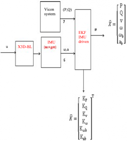
It is convenient to describe this state-space vector not only in the earth frame, but also in a rotating local body frame. The earth fixed is the inertial frame seen through the Vicon-MX system and the body frame is assumed as the rotating frame following the attitude of the quadrotor (seen by the IMU sensors).
This form is also required in calculating the model based controllers. Where: the state $X=\left[\begin{array}{llll}{P} & {q} & {V} & {\omega}\end{array}\right]^{T}$, P: position in earth frame, q: the orientation represented by the quaternion ( earth frame), V: translatory velocity (body frame), $\omega$: angular velocity (body frame).
Saripoalli et al. [14] suggest to append the model state with six extra states to estimate the offset of the gyrometer and accelerometer to compensate for these in the model.
The equivalent state vector now contains: the bias on angular velocity (in the body frame) ($\omega_{b}$) and the bias on acceleration (in the body frame) ($a_{b}$). The state matrix could be then written as:
$\begin{aligned} x &=\left[\begin{array}{llllll}{} & {P} & {q} & {v} & {\omega} & {\omega_{b}} & {a_{b}}\end{array}\right]^{T} \\=&\left[\begin{array}{cccc}{x y z} & {q_{0} q_{1} q_{2} q_{3}} & {v_{1} v_{2} v_{3} \omega_{1} \omega_{2} \omega_{3} \omega_{b 1} \omega_{b 2} \omega_{b 3} a_{b 1} a_{b 2} a_{b 3}}\end{array}\right]^{T} \end{aligned}$ (9)
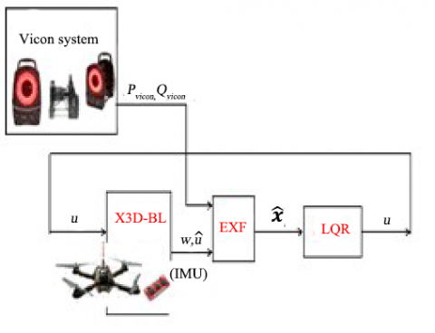
The main reason to use Helicopters instead of fixed wing version is their capabilities to hover around a chosen area. This assumption makes that a quadrotor is usually required to be stabilized around hover in his most operational journey. Thus, a linear state space model around the hovering operating point is set up by the identification of the nonlinearity and using the first order Taylor approximation. For the tracking purpose, an LQR controller is applied in tests (Figure 1).
Figure 1. EKF-IMU Driven with the sensors fusion for the quadrotor closed loop control
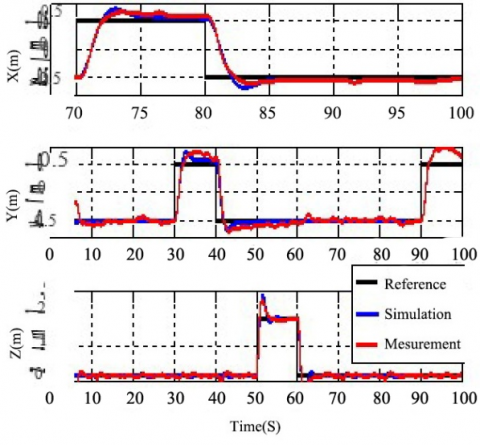
In this paragraph we would like to show how the adopted model was able to estimate successfully the state matrix based on the IMU sensors and the motion tracker updating. The following results are based on the recorded data during the indoor flight. The scenario for the present trajectory starts from the origin ((x,y,z)=(0,0,0)). For the tests, three steps references are sent to the quadrotor: At the moment (t=0), it is desired to reach the position z= -1m. The sign minus here indicate that the reference in the earth frame is pointed from the body to the ground. This is why the z position is always seen negative during the navigation. The following references are translations made on X-axis from 0 to -0.5m then to +1m respectively during the instants (t=3sec, x=-0.5m/ t=3.5second x=+1m).
In Figure 2, it is depicted that the model is well tracking the real position measured by the Vicon-MX system. During the transient phases some drifts in the estimation are noticed and corrected immediately during the update estimation with the Vicon-MX system.
Figure 2. X3D-BL quadrotor Model validation: Simulation vs. Measurements made by the Vicon MX for a set of references on OX, OY, OZ
In this section, this model issued from experiment tests is adopted to generate the model based residuals function under a sensor fault occurrence. Therefore, the corresponding operating-point will be kept near hover to exclude the changing due to the model nonlinearity. We would like here to generate a residual function capable to trigger the fault alarms whenever one sensor of the IMU is subject of fault situation.
A special focus is given herein to the Kalman Gain Matrix (KGM) during the sensor fault scenario. The changes in this matrix are evaluated during the healthy navigation (as a reference) to compare it later with the new matrix generated with respect to the faulty situation in the IMU.
In Table I, the matrix $\boldsymbol{Z}_{\boldsymbol{k}}$ gathers the measurements from the Vicon-MX system and from the Inertial measurement unit (IMU),
$Z=\left[P_{v i c o n} q_{v i c o n} a_{I M U} \omega_{I M U}\right]^{T} \\
=\left[\begin{array}{lllllllll}
{x y z} & {q_{0}} & {q_{1}} & {q_{2} q_{3}} & {a_{1}} & {a_{2}} & {a_{3}} & {\omega_{1} \omega_{2} \omega_{3}}
\end{array}\right]^{T}$ (10)
Combined with the estimated state $\widehat{\boldsymbol{x}}_{k}^{+}$ in (7) & (9), the kalman gain matrix is then:
$\boldsymbol{K}=\left[\begin{array}{ccc}{\mathrm{k}_{1,1}} & {\dots} & {\mathrm{k}_{1,13}} \\ {\vdots} & {\ddots} & {\vdots} \\ {\mathrm{k}_{19,1}} & {\dots} & {\mathrm{k}_{19,13}}\end{array}\right]$ (11)
Each state measured in $\boldsymbol{Z}_{\boldsymbol{k}}$ is linked to a column of the KGM. Thus, the matrix could be seen as:
$K=\left[K_{\text {Pvicon }} \quad k_{\text {qvicon}} K_{a_{I M U}} K_{\omega_{I M U}}\right]^{T}$ (12)
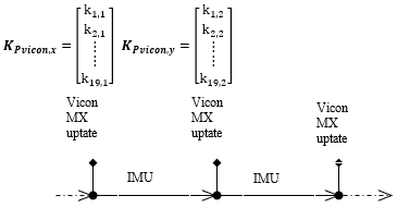
where, also: $K_{\text {Pvicon}}=\left[\boldsymbol{K}_{\text {Pvicon}, x} \boldsymbol{K}_{\text {Pvicon}, \boldsymbol{y}} \boldsymbol{K}_{\text {Pvicon}, z}\right]^{T}$ are the Kalman gains related to the x,y,z position measured by the Vicon-MX system and:
$\boldsymbol{K}_{\text {Pvicon, } \boldsymbol{x}}=\left[\begin{array}{c}{\mathrm{k}_{1,1}} \\ {\mathrm{k}_{2,1}} \\ {\vdots} \\ {\mathrm{k}_{19,1}}\end{array}\right] \boldsymbol{K}_{\text {Pvicon }, \boldsymbol{y}}=\left[\begin{array}{c}{\mathrm{k}_{1,2}} \\ {\mathrm{k}_{2,2}} \\ {\vdots} \\ {\mathrm{k}_{19,2}}\end{array}\right] \\ \boldsymbol{K}_{\text {Pvicon}, \boldsymbol{z}}=\left[\begin{array}{c}{\mathrm{k}_{1,3}} \\ {\mathrm{k}_{2,3}} \\ {\vdots} \\ {\mathrm{k}_{19,3}}\end{array}\right]$ (13)
Thirteen columns are generated on the KGM over nineteen rows in each according to the estimated state matrix (Figure 3).
Figure 3. Extraction of the Kalman gain Matrix for evaluation during the estimation process
5.1 Update time slots of the state matrix
The Motion Tracker LAB is substituting the constellation of satellites such as the global positioning system (GPS). The updating measurements (from the Vicon-MX measurements) are sent once a specific time slot. Between two updating points, the estimated states are based only on the IMU sensors and the prior estimation (Figure 4).
The estimations come very close to the measurements at the steady state and then the gain matrix will be also steady and close to an operational matrix [15]. During the Vicon-MX updating, the drift due to the noise in the IMU measurements is compensated. This will keep the quadrotor inside a cube of certainties and avoids the growth of errors due to the IMU noise.
However, the Vicon-MX measurements will cause a jump in the K matrix parameters if there is a difference between the last estimated state based on the IMU and the new updating based on the Vicon-MX. This correction is also seen as a low frequency updating of the Kalman gain. Usually, with a good model of the system and after the transient state, this variation in the KGM is inside a band with narrowness depending on the updating time slot.
Figure 4. Time slot updating of the estimated states
5.2 Sensor fault scenario
The error in measurement will drive the quadrotor out of his planned journey with the thought that the overall platform is well following its trajectory. A fault in the measurements could be seen as a new $Z_{k}$ matrix. This matrix will be denoted as Z(f)k and will substitute $Z_{k}$ in (7). The resulting matrix of the sensor fault is the new form of measurement during the fault scenario and depends essentially on the fault type. The new state equation will be then:
$\hat{x}_{(f) k}^{+}=\hat{x}_{(f) k}^{-}+K_{k}\left(z_{(f) k}-H_{k}^{[1]} \hat{x}_{(f) k}^{-}\right)$ (14)
Along with this situation, the controller is following the false measurement believing that the references are well tracked. When a new updating of the Vicon-MX is received, a visible difference is noticed between the updated states and the new estimations.
Let´s note $K_{v i c}$: the Kalman gain augmented to comply with the updating states under a sensor fault situation.
$x_{k}^{+}=x_{k(f)}^{-}+K_{v i c}\left(z_{v i c o n ~ u p d a t e}-H_{k}^{[1]} x_{k(f)}^{-}\right)$ (15)
To comply the actual situation, the second term of (14) involving the false measurements tends to be corrected through a new Kalman Gain evaluation in (15).
The controller now receives the real state and will struggle to correct his trajectory.
The outputs from the Vicon-MX system are absent and the measurements are only drawn from the IMU sensors, the controller receives again the false measurements.
Fortunately and thanks to the integration of the false measurement, the estimated positions and attitudes will be pushed gradually and not roughly to the wrong states since the positions (x, y, z) and the attitudes $(\varphi, \theta, \psi)$ are the second and first integration of the accelerations $a_{x, y, z}$ and angular velocity $\omega=[\dot{\varphi}, \dot{\theta}, \dot{\psi}]$ respectively. As a result, the new evaluated positions will not drift to wrong values spontaneously.
During the updating of the measurement the new estimated state is calculated again from (7) and, the new residuals will induce a new covariance matrix $P_{k}^{-}$.
Looking to the updating matrix of the Kalman gain (6), one could deduce that the new available data from the covariance matrix $P_{k}^{-}$ will stimulate a rough variation on some Kalman gains relatively to the state under sensor fault effect. When the estimation process switches to the faulty IMU, (14) will be active. The new estimations are then based on the false measurements. The fact that the fault is in the accelerometers or the Gyrometers, the resulting estimated states of the position (x, y, z) and attitude $\left(q_{0}, q_{1} q_{2} q_{3}\right)$ are changing in an integration rate manner (gradually). As a result, the corresponding Kalman gain will also receive a slow change.
After few updating of the state matrix, with a quick impact of the Vicon-MX and slow impact of the sensor fault in the IMU, the system will be corrected gradually in an equivalence to a new system model. Consequently, the overall Kalman gain matrix is carried to the new steady state around the uncorrected state.
The non-linear form of the Kalman gain matrix typically results in a matrix being highly changing over a small time interval. Therefore, one should look for a function to evaluate its behavior in fault free and fault evolution (in one or more sensors) according to the overall changes and based on the instantaneous variations. It is noticed from (12) and (13) that the gains of the same column are linked to the same sensor, therefore we propose to fuse together the columns of KGM in the root square of the absolute column sum 2-norm. as:
$\mathcal{N}_{p j}=\left\|k_{i, j}\right\|_{i=1: n}=\sqrt[2]{\sum_{1}^{n} k_{i, j}^{2}} \quad j=1: m$ (16)
In this manner, the calculated norms $\mathcal{N}_{p_{j}}$ will show an overall description of the gains linked to each specific column corresponding to the related sensor, no matter the direction or the sign of each gain.
We wish to employ this matrix norm in the residual function based on the KGM behavior.
However, due to the high frequency changes of this matrix, the absolute column sum 2-norm is also a high frequency changing (Figure 5).
To filter this new function, it is more convenient to check a set of gain data along with a sufficient time interval. The influence of sample variability in the KGM may seriously affect the calculated norms $\mathcal{N}_{p j}$, and generate an overpassing spikes that could deteriorate the decision of the alarm against any malfunctioning.
To avoid these undesirable spikes in the Kalman gain norm, one could notice that the very hard changes are originally coming from the updating through the GPS (or the Motion tracker) during the fault free estimation. Therefore, we choose the updating time interval for the absolute column sum 2-norm filter similar to the updating time of the navigation. The mean value over the updating interval will suppress the high frequency variability in the KGM-Norm and shows an overall tendency of the absolute column sum 2-norm function. In fact, this mean value evaluation is a kind of low pass filtering that describes the tendency of the system model without considering the instantaneous responses.
$\overline{{{N}_{{{p}_{J}}}}}$ notes the mean value of the absolute column sum 2-norm function. The change in $\overline{{{N}_{{{p}_{J}}}}}$ reflects an overall change in the system and may trigger the fault alarm in case of over passing of the threshold. The initial data of $\overline{{{N}_{{{p}_{J}}}}}$ corresponding to the healthy system will be stored in memory as reference for the health checking. Due to the low frequency evaluation of the Norm $\overline{{{N}_{{{p}_{J}}}}}$, the variation in $(\overline{{{N}_{{{p}_{J}}}}})$ is assumed as the residual function $\Delta \overline{{{N}_{{{p}_{J}}}}}$. These residuals are to satisfy a desirable compromise between a maximum sensitivity to the faults and a minimum sensitivity to the disturbances (measurement noises, GPS update).
Figure 5. The Norm-2 of the Kalman gain KP relative to the measured positions (X)
In the present section, the Norm Kalman gain $\overline{{{N}_{{{p}_{J}}}}}$ is evaluated during a fault free flight then compared to the same evaluation during a sensor fault occurrence in one of the Inertial Measurement Unit.
To check the effectiveness of the method, the following cases are considered:
a) Changes in the input references and check the changes in $\overline{{{N}_{{{p}_{J}}}}}$:
a-1 step change in reference in position X
a-2 slope change reference in position X
b) A fault occurrence in one accelerometer (on X-axis as an example) in an additive fault:
b-1 step additive fault (rough variation in the measurement)
b-2 a slope additive fault (smooth variation in the measurement)
7.1 Test 1. Navigation sensor fault free
7.1.1 Step variation in command reference
We would like to inspect the behavior of this function $\overline{{{N}_{{{p}_{J}}}}}$ when the quadrotor moves from one hovering point to another.
With respect to Z matrix elements in (10).
$\overline{{{N}_{{{p}_{1..3}}}}}$ are the mean value of the norm- (MVN) related to all the changes due to the (x, y, z)-positions $\overline{{{N}_{{{p}_{4..7}}}}}$ are the MVN related to the quaternion (attitude seen in the quaternion representation).
$\overline{{{N}_{{{p}_{8.。10}}}}}$ and $\overline{{{N}_{{{p}_{11..13}}}}}$ are respectively the MVN related to the gyrometers $(\varphi, \theta, \psi)$ and the accelerometers ($\left(a_{x}, a_{y}, a_{z}\right)$.
To display the results and due to the number of resulting figures (up to 13), only $\overline{{{N}_{{{p}_{1..3}}}}}$ and $\overline{{{N}_{{{p}_{4..7}}}}}$ will be considered.
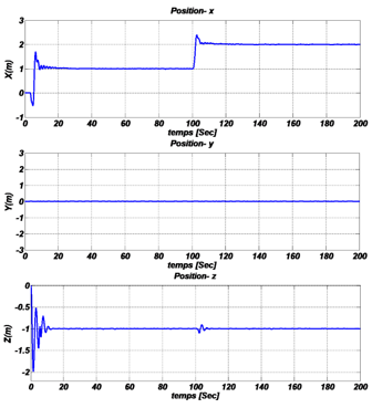
a)At t=0 from the origin (x,y,z)=(0,0,0) a step for the thrust is send as Zref to the controller, to take off from z=0m to z=-1m (seen in the earth frame).
At: t= 3sec a reference sent to X as Xref= -0.5m
At: t=3.5 sec a reference sent to X as Xref= +1m
At: t=50sec a reference sent to X as Xref= -1m
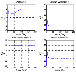
After the first transient interval [0sec 8sec] when the quadrotor moves from the ground to the hovering position (z=-1, y=0, x=1) (Figure 6), the changes in $\overline{{{N}_{{{p}_{J}}}}}$ are due to the transient states when the UAV follows the references from the ground position to the desired hovering position (Figure 7). These will disappear as soon as the quadrotor reaches his steady state.
Figure 6. Time response of the quadrotor on the Cartesian positions for a step variation on the X reference from Xref =+1m to Xref =+2m at time t=100sec
It is clear that all the $\overline{{{N}_{{{p}_{J}}}}}$ elements become almost fixed in constant values after this transition (Figure 7). A new reference to the x position from +1m to -1m is set at the moment t=50sec, another transient response reflecting this difference between the reference and the actual position will come into sight on $\overline{{{N}_{{{p}_{J}}}}}$.
When the Kalman gain reaches again his steady state, we notice again that $\overline{{{N}_{{{p}_{J}}}}}$ becomes steady and tends again to the same values seen before. This is an interesting result that all norms of the Kalman gain matrix will come back again to the old values.
Figure 7. Test.1.a. Kalman gain matrix behavior against a step variation on a reference of command
7.1.2 Smooth variation in command reference
The impact on $\overline{{{N}_{{{p}_{J}}}}}$ is considered when the quadrotor is moving between two points out of hovering navigation case. For constant velocity a slope reference will be applied to the controller from t=50sec with a slope variation of 0.2m/sec.
For convenience, only three among thirteen curves are shown (Figure 8). First in the top left corner of Figure 8, the time response of the Cartesian position OX for a smooth reference slope equal to 0,02m/s on X-axis at t=50sec to reach X=2m in 50sec. then, the Norm -2 of the Kalman gain relative to the measured positions (X,Y,Z). It is noticed one more time that $\overline{{{N}_{{{p}_{J}}}}}$ is not affected by the navigation.
As a result, the effect of the moving from one hovering position to another and the translation cases (which reflect the general case) does not affect the norm of this matrix.
Figure 8. Test.1.b. Time response of the cartesian position OX and The mean Norm -2 of the Kalman gain relative to the measured positions (X,Y,Z)
7.2 Test 2. Quadrotor navigation under sensor fault occurrence
Since the KGM is insensitive to the references change for a full operation in different maneuvers. We are going to inspect here the effect of a sensor fault on the gain matrix (KGM).
7.2.1 Additive fault in step
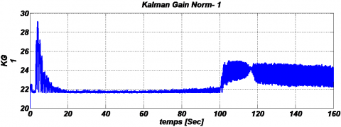
Here, an additional portion is introduced into the measured acceleration on the X-axis as an additive fault. $\operatorname{acc} x_{\text {error}}=+1 \mathrm{m} / \mathrm{s}^{2}$ to provoke a sensor fault at the moment t=100sec during the hovering of the quadrotor.
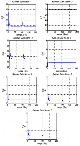
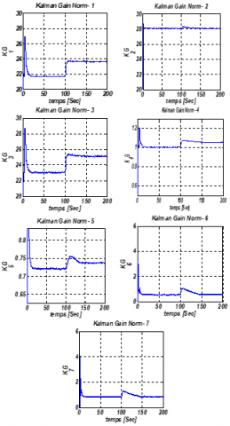
Figure 9 illustrates the mean value of the norm on each column with respect to $(P, q)$ in the KGM and its behavior during the sensor fault case. As depicted from Figure 9, it can be seen that the mean value of the $K G_{1}$ and $K G_{3}$ are clearly affected by the fault occurrence where the $K G_{2}$ has less reaction to the fault. This is very close to be true since the x-accelerometer would affect the updating state on X position and vey less effect on Y-axis. But why $K G_{3}$ is affected?
During the hovering flight, the lifting force is on Z-axis and the thrust becomes steady to keep the platform around the hovering -position. When a translation on X-axis is sensed due to the wrong measurement, the controller develops an adverse pitch angle to correct the quadrotor flight. This manoeuver will affect the total force vector and the thrust will assign a portion to the translator movement. Therefore, the lifting force becomes less to keep Z-position near to the reference and the estimation of the Z-position is seen as going less than the desired reference. At this moment, the controller starts again to correct this z position by pumping more thrust to the rotors. During the Vicon-MX update, the controller receives the real state of z-position which was affected by the additional pitch angle and then tends to correct it again. Thus, the z-position state is swinging also between two limits, one due to the X-accelerometer extra portion issued from the fault on the sensor and the other due to the Vicon-MX updating. In the same manner, some changes that reflect the occurrence of the fault on the considered sensor are depicted also on the Mean value of the KGM with respect to the quaternion, Figure 9.
When applying a similar faults on the other two accelerometers on Y-axis and Z-axis, the KGM shows also a sensitivity to the sensor fault.
Figure 9. Mean Norm-2 of Kalman gain matrix evaluation (columns 1 to 7) during a sensor fault in Acc on x-axis at t=100sec
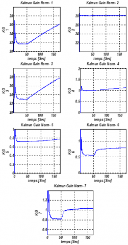
7.2.2 Additive fault in slope
In Figure 10 when applying a slow deviation in the accelerometer measurement, $(\overline{{{N}_{{{p}_{J}}}}})$ start also to sense this false measurement with the same shape of the deviation.
It is a very interesting property that the Kalman gain matrix norm is responsive to the additive fault in a sensor of the IMU. We applied a similar tests on the rest of the sensors and $\overline{{{N}_{{{p}_{J}}}}}$ present a good sensitivity to the fault occurrence in a sensor and less sensitivity to the normal navigation conditions. This technique exploits only the change in the Gain matrix when an abnormal behavior occurs during the navigation no matter the nature of the fault. It is completely independent of the kind of the fault in the sensor. Therefore, this property could be extended to other types of faults such as the multiplicative fault or stack in point fault where the sensor is planted to a specific measurement even the real states are changing.
Figure 10. Mean Norm-2 of Kalman gain matrix evaluation (columns 1 to 7) during a sensor fault in slope variation of 0.02m/s in Accelerometer on x-axis at t=50sec
The fact that the changes in Mean values of Kalman Gain Norm-2 $(\overline{{{N}_{{{p}_{J}}}}})$ are steady with very less variation, the use of this property as residual function to detect changes or malfunctioning in the sensors will yield a decision to trigger the alarm free of the disturbances effect. The Kalman Gain Matrix could be then used as a new alternative to detect the sensor fault occurrence. Unlike the residuals based on a set of Kalman filters used extensively, this proposed function will benefit from the set of Kalman gains of only one Kalman filter to detect the sensor fault. This reduction yields to a considerable minimization of both, time of calculation and the onboard memory size. Assuming that the mean values of Kalman Gain Norm-2 $\overline{{{N}_{{{p}_{J}}}}}$ during the healthy sensors case as the references in the residual generation, this low frequency analysis will return in residuals where, the effects due to the high frequency disturbances and sensor noise are attenuated.
The future work will consider an analysis of different behaviors of each Kalman gain related to a set of scenarios of possible sensor faults in the inertial measurement unit so as to establish an algorithm capable to isolate the faulty sensor.
|
ab |
The bias on acceleration (in the body frame) |
|
$\mathbf{H} k$: |
Matrix connect the states to the to the measurement |
|
KPvicon |
The Kalman gains related to the x,y,z position measured by the Vicon-MX system. |
|
Kvic: |
The Kalman gains related to quaternion attitude measured by the Vicon-MX system. |
|
k and k-1: |
The indices indicate the current sample and the previous sample respectively |
|
P: |
Position in earth frame, |
|
Pk|k-1 |
Error covaiance from k-1 to k |
|
Pk |
The estimation covariance, |
|
q: |
The orientation represented by the quaternion |
|
$Q k$: |
Noise covariance matrix |
|
X: |
The state matrix, |
|
$\hat{\mathbf{x}}_{\mathbf{k}}$ |
The priori estimates of the state vector |
|
$\widehat{\boldsymbol{x}}_{\boldsymbol{k}}^{+}$: |
The estimated state vector at the k sample |
|
$\dot{x}_{k | k-1}$ |
Residuals between the real and estimation states |
|
V: |
Translatory velocity (body frame), |
|
Z: |
The sensors outputs matrix |
|
Zk: |
Measurement matrix at k sample |
|
$Z(f) k^{:}$ |
Fault in the measurements |
|
Greek symbols |
|
|
φ |
Rotation angle around OX axis |
|
θ |
Rotation angle around OY axis |
|
Ψ |
Rotation angle around OZ axis |
|
[φ θ Ψ] |
The Euler angles. |
|
ω: |
Angular velocity (body frame). |
|
ωb: |
The bias on angular velocity (in the body frame) |
|
$w k \sim \mathcal{N}(0, Q k)$ |
Gaussian noise with zero mean value and $Q k$ covariance |
|
Φ(X): |
Evolution matrix of the state X |
|
Φ[1] (X): |
Linearization of Φ(X) |
|
$\overline{{{N}_{{{p}_{J}}}}}$ |
The mean value of the absolute column sum 2-norm function of the Kalman matrix. |
|
$\Delta \overline{{{N}_{{{p}_{J}}}}}$ |
The residual function of the variation in $\overline{{{N}_{{{p}_{J}}}}}$ |
|
Subscripts |
|
|
+ and -: |
Indicate a priori or a posterior estimate respectively |
|
([1]) |
Denotes the 1st order linear Taylor approximation of a nonlinear function. |
[1] Frank, P.M., Ding, X. (1997). Survey of robust residual generation and evaluation methods in observer-based fault detection systems. Journal of Process Control, 7(6): 403-424. http://dx.doi.org/10.1016/S0959-1524(97)00016-4
[2] Ding, S.X., Zhang, P., Ding, E.L., Frank, P.M., Sader, M. (2003). Multi-objective design of fault detection filters. 2003 European Control Conference (ECC), Cambridge, UK, pp. 1378-1383. http://doi.org/10.23919/ECC.2003.7085150
[3] Yu, D., Shields, D.N. (1996). A bilinear fault detection observer. Automatica, 32(11): 1597-1602. http://dx.doi.org/10.1016/S0005-1098(96)00111-2
[4] Huang, C., Yi, G.X., Zeng, Q.S., Hu, L., Xu, Z.Y. (2019). Design and software implementation of a navigation accuracy evaluation based on error model solution. Instrumentation Mesure Métrologie Journal, 18(3): 267-273. https://doi.org/10.18280/i2m.180306
[5] Napolitano, M., An, Y., Seanor, B. (2000). A fault tolerant flight control system for sensor and actuator failures using neural networks. Aircraft Design, 3(3): 103-128. http://dx.doi.org/10.1016/S1369-8869(00)00009-4
[6] Liu, J., Wang, J.L., Yang, G.H. (2005). An LMI approach to minimum sensitivity analysis with application to fault detection. Automatica, 41(11): 1995-2004. https://doi.org/10.1016/j.automatica.2005.06.005
[7] Napolitano, M.R., Windon, D.A., Casanova, J.L., Innocenti, M., Silvestri, G. (1998). Kalman filters and neural-network schemes for sensor validation in flight control systems. IEEE Transactions on Control Systems, 6(5): 596-611. http://dx.doi.org/10.1109/87.709495
[8] Deng, Z.L., Gao, Y., Mao, L., Li, Y., Hao, G. (2005). New approach to information fusion steady-state Kalman filtering. Automatica, 41(10): 1695-1707. http://dx.doi.org/10.1016/j.automatica.2005.04.020
[9] Halder, A., Chakravarty, D. (2018). Investigation of wireless tracking performance in the tunnel-like environment with particle filter. Mathematical Modelling of Engineering Problems Journal, 5(2): 93-101. https://doi.org/10.18280/mmep.050206
[10] Nguyen, H.V., Berbra, C., Lesecq, S., Gentil, S., Barraud, A., Godi, C. (2009). Diagnosis of an inertial measurement unit based on set membership estimation. 2009 17th Mediterranean Conference on Control and Automation, Thessaloniki, Greece, pp. 211-216. http://dx.doi.org/10.1109/MED.2009.5164541
[11] Khebbache, H., Sait, B., Bounar, N., Yacef, F. (2012). Robust stabilization of a quadrotor UAV in presence of actuator and sensor faults. International Journal of Instrumentation and Control Systems (IJICS), 2(2): 53-67. http://dx.doi.org/10.5121/ijics.2012.2205
[12] Bisgaard, M. (2007). Modeling, estimation, and control of helicopter slung load system. Ph.D. Thesis., Depat. Electronic Systems Section for Automation and Control. Aalborg Univ., AAU. Danmark.
[13] Jun, M., Roumeliotis, S.I., Sukhatme, G.S. (1999). State Estimation of an autonomous helicopter using kalman filtering. Proceedings 1999 IEEE/RSJ International Conference on Intelligent Robots and Systems. Human and Environment Friendly Robots with High Intelligence and Emotional Quotients (Cat. No.99CH36289), Kyongju, South Korea, pp. 1346-1353. http://dx.doi.org/10.1109/IROS.1999.811667
[14] Saripoalli, S., Roberts, J.M., Corke, P.I., Buskey, G., Sukhatme, G.S. (2003). A tale o-f two helicopters. Proceedings 2003 IEEE/RSJ International Conference on Intelligent Robots and Systems (IROS 2003) (Cat. No.03CH37453), Las Vegas, NV, USA, pp. 805-810. http://dx.doi.org/10.1109/IROS.2003.1250728
[15] Heredia, G., Ollero, A., Bejar, M., Mahtani, R. (2008). Sensor and actuator fault detection in small autonomous helicopters. Mechatronics, 18(2): 90-99. http://dx.doi.org/10.1016/j.mechatronics.2007.09.007