Abdelhak Abdou* | Tarik Bouchala | Bachir Abdelhadi | Amor Guettafi | Azzedine Benoudjit
OPEN ACCESS
This paper puts forward a novel nondestructive method to measure the coating thickness of aeronautical construction materials (e.g. Al, AU4G, Ti and Inox 304L) using the eddy current. First, the forward model of the coupled electric field method was adopted to facilitate the eddy current measurement the coating thickness. The forward model was applied in Matlab simulation. Based on the simulation results, the authors examined the effects of nonconductive coating thickness on sensor impedance component such as amplitude, resistance and reactance. On this basis, an inverse algorithm was developed and coupled with the forward model, and verified through experiments. The results show that our method can measure the coating thickness of aeronautical construction materials rapidly at a high precision. The method has great potential for automated industrial applications.
eddy current sensor, coating thickness, inverse problem, coupled electric field method, metal sheet
In the field of aeronautics, aircraft are periodically subject to inspection and maintenance operations, as in the case of Algeria's aircraft maintenance division. In the nondestructive testing workshop, eddy current technique is widely used for evaluating and controlling the relevant parts of aircraft. Among these applications, the non-conductive coating thickness measurement [1]. So, dielectric coatings such as paint and varnish are used in aeronautic construction for heat-shielding, heat resisting, anticorrosive [2]. In industrial automatic application, several iterative inversion methods are used to accomplish this objective. In general, the flowchart constitutes an iteration buckle containing the forward model associated to an inversion algorithm [3-4]. We recall that analytical forward method of Dodd and Deeds gives the exact solution but the skin and the proximity effects in the exciting coil turns are neglected [5]. On other hand, the finite element method (FEM) is applicable to any complex devices without restrictions, but it’s relatively slow in comparison to the analytical ones. For this reason, our effort is mainly focused on the application of the coupled electric field method (CEFM) that we have recently developed and performed because itis fast and can take into consideration both skin and proximity effects [6]. In this paper, our goal is to associate the coupled circuit method and a new deterministic optimization method that we have recently developed for measuring the non-conductive coating thickness of Al, AU4G, Ti and Inox-304L sheet metals [7].
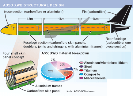
A coating thickness meter is a scientific instrument for measuring the thickness of layers on a base material called substrate or support. So, coating thickness measurement is a very useful discipline in materials science. Thickness of conductive or nonconductive coating thickness is one of the essential criteria for characterizing a coating; a minimum layer thickness on a part is required to ensure physical, electrical, mechanical or aesthetic properties [1]. Typical application areas are the automotive, microelectronics and aeronautics industries. In aircraft and aeronautical domains, several sheet metal materials such as Al, AU4G, Ti and stainless steel 304L with coating layer are used to ensure resistance to mechanical thermal and chemical constraints, as shown in Figure 1.
Figure 1. Aeronautic construction materials
The plane cockle is made, in majority, of aluminium alloys formed by aluminium mixed respectively with copper and zinc. Aluminium is used in general because its volume density is very weak, what presents an advantage in aeronautics. Indeed, more the plane is light, it consumes less. Aluminium is also very appreciated its good resistance for corrosion. Aluminium is easily malleable what makes the construction of different easier [8, 9].
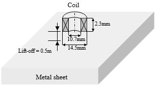
In our study, the metal presents a flat surface with thin nonconductive coating. In a concrete study, when using eddy current to measure non conductive coating thickness, it is important to ensure that the other factors are kept under control. A pancake-type probe formed of coil used whose axis is perpendicular to the surface of the tested piece [10-16]. This type of sensor is used for flat surface inspections, Figure 2. In our study, we neglect the parameters that affect commonly coating thickness measurement such as: Edge effects, curvature, cleaning of surface and perpendicularity of the sensor probe.
Figure 2. Studied device
The geometrical and physical characteristics are given in Table 1.
Table 1. Characteristics of the studied device
|
Coil |
|
|
Current intensity Frequency Inner radius Length High |
0.04A 10 kHz 5.35 [mm]. 2.35 [mm]. 2.3 [mm]. |
|
Plate |
|
|
Thickness Electric conductivity Magnetic permeability |
2 [mm]. That of Al, Inox 304L, Ti 1 |
The electromagnetic phenomenon intervening in eddy current non-destructive systems is described by the following generalized punctual Eqns. [9-15].
$\frac { 2 \pi r ( p ) } { \sigma } J ( p ) + \mu _ { o } r ( p ) G ( p , q ) \frac { d I ( q ) } { d t } = u ( p )$ (1)
$G ( p , q ) = \sqrt { \frac { r ( p ) } { r ( q ) } } E ( k ( p , q ) )$ (2)
$E ( k ) = \frac { \left( 2 - k ^ { 2 } \right) E _ { 1 } ( k ) - 2 E _ { 2 } ( k ) } { k }$ (3)
$k ( p , q ) = \sqrt { \frac { 4 r ( p ) r ( q ) } { ( r ( p ) + r ( q ) ) ^ { 2 } + ( z ( p ) - z ( q ) ) ^ { 2 } } }$ (4)
where,
G(p,q) is called Green’s function and represents the response of the system at a point p(r,z) to Dirac’s distribution located at a point q.
E1(k) and E2(k) are respectively the first and the second species of the Legendre elliptic function [9].
w is the pulsation.
r(p) and r(q) are the radial coordinate of the point p and q, respectively.
z(p) and z(q) are the axial coordinate of the point p and q, respectively.
Eq. (2) expresses the creation of the current intensity I(p) at a point p of electric conductivity s(p) under the influence of the voltage u(p) applied at this point, and the current intensity I(q) situated in q.
The above equations describe only the electromagnetic effect of one point upon another. To realize the electromagnetic contribution of the complete domain W upon point p, Eq. (1) is rewritten in the following form:
$\frac { 2 \pi r ( p ) } { \sigma ( p ) } J ( p ) + j \omega \mu _ { 0 } r ( p ) \iint _ { \Omega } G ( p , q ) J ( p , q ) d \Omega = u ( p )$ (5)
In our case, we need to express eddy current probe impedance variation caused by the presence of the conductive material, according to its thickness Ec and electric conductivity σ.
The current density J(p) can be expressed according to the electric field E(p) as follows:
$\left\{ \begin{array} { l } { J ( p ) = \sigma ( p ) E ( p ) } \\ { I ( p ) = s ( p ) \sigma ( p ) E ( p ) } \end{array} \right.$ (6)
S(p) is the cross section of the turn p.
By introducing the transformation of equation set (6), equation (5) leads to equation (7). We have named this latter the generalized coupled electric field equation:
$2 \pi r ( p ) E ( p ) + \mu _ { o } r ( p ) \iint _ { \Omega } G ( p , q ) \sigma ( p ) E ( p ) d \Omega = u ( p )$ (7)
The next sections will be devoted to the modeling of axi-symmetrical configuration by applying Eq. (6) on the exciting coil region and Eq. (8) on the tested conductive piece.
In the present study, the metal sheet is considered as a flat surface with or without a thin nonconductive coating. In fact, the exciting coil of domain Ωo delivers a sinusoidal magnetic field that induces eddy current in a massive metal sheet of domain Ωc.
In view of the fact that the system is axially symmetric, the magnetic field calculation is performed only in a half domain. In addition, since the depth penetration is relatively deep in comparison to the turn’s section radius, we admit that the current density distribution in this section is uniform. Therefore, the number of elements on the sensor is equal among turns of both reels. In other words, the number of elements is No distributed on Nor on the radial direction and Noz on the axial direction. The inspected metal sheet is subdivided into $N _ { c } \left( N _ { c\, r} , N _ { c \,z } \right)$ elements as illustrated in Figure 3.
Figure 3. Two-dimensional geometry and meshing
The domain W is divided into two active regions: the one of the sensor coils is denoted Wo while the other region of the piece is denoted Wc. The presence of induced currents in the piece influences the source current density Jo. To express this influence, we apply Eq. (5) to both coil and piece domains respectively.
$\frac{2\pi {{r}_{o}}\left( {{p}_{o}} \right)}{{{\sigma }_{o}}({{p}_{o}})}{{J}_{o}}\left( {{p}_{o}} \right)+j\omega {{\mu }_{o}}{{r}_{o}}\left( {{p}_{o}} \right)\iint\limits_{{{\Omega }_{o}}}{G\left( {{p}_{o}},{{q}_{o}} \right)\,{{J}_{o}}\left( {{q}_{o}} \right)\ d{{\Omega }_{o}}}+j\omega {{\mu }_{o}}{{r}_{o}}\left( {{p}_{o}} \right)\iint\limits_{{{\Omega }_{c}}}{G\left( {{p}_{o}},{{q}_{c}} \right)\,{{J}_{c}}\left( {{q}_{c}} \right)\ d{{\Omega }_{c}}}=u({{p}_{o}})$ (8)
According to Figure 2, when the previous domains Wo and Wc are meshed into No and Nc elementary loops respectively and by considering that the sensor is subjected to a total voltage U, Eq. (8) becomes:
$\sum\limits_{{{p}_{o}}=1}^{{{N}_{o}}}{\frac{2\pi \,{{r}_{o}}\left( {{p}_{o}} \right)}{{{\sigma }_{o}}({{p}_{o}})\,{{S}_{o}}({{p}_{o}})}{{I}_{o}}}+j\omega {{\mu }_{o}}{{I}_{o}}\sum\limits_{{{p}_{o}}=1}^{{{N}_{o}}}{{}}{{r}_{o}}\left( {{p}_{o}} \right)\sum\limits_{{{q}_{o}}=1}^{{{N}_{o}}}{G\,\left( {{p}_{o}},{{q}_{o}} \right)}+j\omega {{\mu }_{o}}\sum\limits_{{{p}_{o}}=1}^{{{N}_{o}}}{{}}{{r}_{o}}\left( {{p}_{o}} \right)\sum\limits_{{{q}_{c}}=1}^{{{N}_{c}}}{G\,\left( {{p}_{o}},{{q}_{c}} \right)\,{{S}_{c}}{{\sigma }_{c}}{{E}_{c}}\left( {{q}_{c}} \right)}=U$ (9)
where, so and ro are respectively the section and the radius of the coil loop, and so is the electric conductivity. G is a function of relative coordinates between elementary loops.
To describe the induced electric field Ec in the massive conductive piece, we apply on its Eq. (8), then we can write:
$2\pi {{E}_{c}}\left( {{p}_{c}} \right)+j\omega {{\mu }_{o}}\sum\limits_{\begin{smallmatrix} {{q}_{c}}=1 \\ {{q}_{c}}\ne {{p}_{c}}\end{smallmatrix}}^{{{N}_{c}}}{G\left( {{p}_{c}},{{q}_{c}} \right){{S}_{c}}{{\sigma }_{c}}{{E}_{c}}\left( {{q}_{c}} \right)}+j\omega {{\mu }_{o}}{{I}_{o}}\sum\limits_{{{q}_{o}}=1}^{{{N}_{o}}}{G\left( {{p}_{c}},{{q}_{o}} \right)}=0$ (10)
where, Sc and rc are respectively the section and the radius of the tested piece loop.
The impedance is the quotient between the voltage U and the exciting current intensity Io. The calculation approach of the impedance variation is very important for material characterization [9]. The impedance variation is the difference between the impedance Z in presence of the piece and the one in free space Zo.
$\Delta Z = Z - Z _ { 0 }$ (11)
From Eq. (9) and relation (11), one can finally deduce the expression of this impedance variation:
$\Delta Z = \frac { j \omega \mu _ { o } } { I _ { o } } \sum _ { p _ { o } = 1 } ^ { N _ { o } } r _ { o } \left( p _ { o } \right) \sum _ { q _ { c } = 1 } ^ { N _ { c } } G \left( p _ { o } , q _ { c } \right) S _ { c } \sigma _ { c } E _ { c } \left( q _ { c } \right)$ (12)
We have also:
$S _ { c } = \frac { E _ { c } T _ { c } } { N _ { c } }$ (13)
$\Delta Z = \frac { j \omega \mu _ { o } L _ { c } } { I _ { o } N _ { c } } \sum _ { p _ { o } = 1 } ^ { N _ { o } } r _ { o } \left( p _ { o } \right) \sum _ { q _ { e } = 1 } ^ { N _ { c } } G \left( p _ { o } , q _ { c } \right) E _ { c } \left( q _ { c } \right) T _ { c } \sigma _ { c }$ (14)
After having accomplished the development of the forward model, the next section will be dedicated to resolve the inverse problem which consists in measuring the coating thickness.
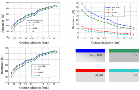
After implanting the coupled circuit method on MATLAB software, we study the effect of non conductive coating thickness on sensor impedance component such as amplitude, resistance and reactance; the coated sheet metal is made of Inox304L, Aluminium, AU4G and Titanium.
From these results, we remark clearly that the resistance variation increases with the increase of coating thickness. Furthermore, greater variations are obtained for high frequencies.
Our objective in this section is not to make a deep analysis of these results because this problem is already treated in previous works, but we want to make in evidence that resistance variation ∆R changes more rapidly in comparison to the reactance variation ∆X. The next section is reserved to exploit the developed forward model for resolving the inverse problem which consists in measuring nonconductive coating thickness.
Figure 4. Impedance variation according to coating thickness for different material type. fr =10Khz
Figure 5. Impedance variation according to coating thickness for different material type. fr. =10Mhz
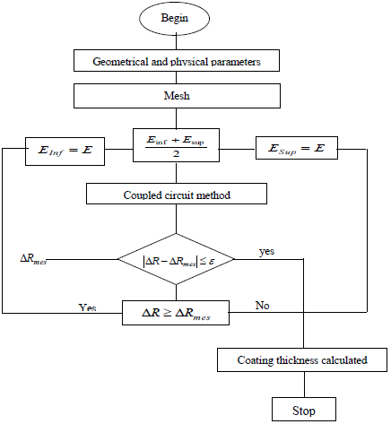
The inverse method that we propose in this contribution is based on the association of the forward developed model and an algorithm researching the inverse problem solution, which is the tested piece coating thickness, from the measured impedance variation [7]. The algorithm exploits the fact that the sensor resistance variation according to coating thickness is an increasing function (∆R=f(E)). While knowing the physical and geometric parameters of the studied system and the starting interval limits (Einf and Esup), successively, by lower and upper coating thickness, the forward model determines the resistance variation corresponding to the intermediate coating thickness (Einf + Esup)/2.
If the calculated resistance ∆R is lower than ∆Rmes, the coating thickness Esup is replaced by (Einf + Esup)/2. Otherwise, if ∆R is greater than ∆Rmes, the coating thickness Esup is replaced by (Einf + Esup)/2. This process is repeated until the difference between ∆R and ∆Rmes becomes lower than the tolerance ($\left| \Delta R - \Delta R _ { \text {mes } } \right| \leq \varepsilon$). These process steps are summarized in Figure 6.
This algorithm presents several advantages such as: the solution is guaranteed in advance if the sought value belongs to the starting interval. Certainly, in the industrial applications the expert knows the starting interval of coating thickness.
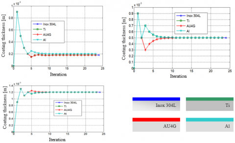
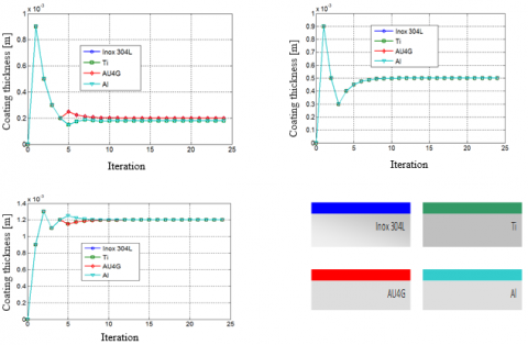
In the following sections, we apply the developed inverse method to determine non-conductive coating thickness of Inox304L, Aluminium, AU4G and Titanium. So, the evolution of the coating thickness, for exciting field frequency 1 kHz and 1 MHz, according to iteration number is shown on Figures 7 and 8. The dielectric coating thickness is about of 0.2 mm, 0.5 mm and 1.2 mm.
Figure 6. Proposed optimization flowchart
Figure 7. Coating thickness for different material type according to iteration. fr =10Khz. fr =10kHz calculated with the proposed algorithm
Figure 8. Coating thickness for different material type according to iteration. fr =10MHz calculated with the proposed algorithm
During this application, we have seen that the values obtained by the proposed method are very precise and closer to desired ones, which shows the robustness of this method. In fact, for all sheet metal type, less than 10 iteration are sufficient to determine coating thickness (0.2 mm, 0.5 mm and 1.2 mm). Also, we know that probabilistic methods such as genetic algorithm is very expensive in computation time because of the high number of objective function evaluations at each iteration. On the other hand, to achieve an acceptable accuracy, the population size must be increased what induce a significant computation time. As a result, the proposed method is more preferred; because it is faster and its performance doesn't change when the calculation is reset, which is not the case for the other stochastic methods [18-21].
In this paper we have exploit the deterministic method that we have recently developed for non-destructive evaluation of coating thickness aircraft construction materials [6]. So, after implementing and running the inversion technique under Matlab environment, the simulation results has shown its rapidity and robustness while making a judicious configuration choice for initial parameters such as initial interval search and tolerance. In fact, while using this algorithm, few iteration numbers are sufficient for real time coating thickness measurement. As future work, we look forward to extend this inversion procedure to characterize the aeronautical metal sheet by introducing its thickness and that coatingan unknown parameters.
[1] Javier, G.M., Jaime, G.G., Ernesto, V.S. (2011). Non-destructive techniques based on eddy current testing. Sensors Journal, 11(3): 2525-2565. https://doi.org/10.3390/s110302525
[2] Bruchwald, O., Nicolaus, M., Frackowiak, W., Reimche, W., Möhwald, K., Maier, H.J. (2016). Material characterization of thin coatings using high frequency eddy current technology. 19th World Conference on Non-Destructive Testing 2016.
[3] Lunin, V.P. (2006). Phenomenological and algorithmic method for the solution of inverse problem of electromagnetic testing. Russian Journal of Nondestructive Testing, 42(6): 353-362. https://doi.org/10.1134/S1061830906060015
[4] Han, W., Que, P. (2005). An improved genetic local search algorithm for defect reconstruction from MFL signals. Russian Journal of Non-destructive Testing, 41(12): 815-821.
[5] Dodd, C.V., Deeds, W.E. (1968). Analytical solutions to eddy-current probe-coil probe problems. Journal of Applied Physics, 39(6): 2829-2839. https://doi.org/10.1063/1.1656680
[6] Amrane, S., Latreche, M.E.H., Feliachi, M. (2010). Coupled circuits model combined with deterministic and stochastic algorithms for the inductor design. International Journal of Applied Electromagnetics and Mechanics, 32(4): 195-206. https://doi.org/10.3233/JAE-2010-1074
[7] Bouchala, T., Abdelhadi, B., Benoudjit, A. (2015). New contactless eddy current non-destructive methodology of electric conductivity measurement. Journal of Non-destructive Testing and Evaluation, 30(1): 63-73. https://doi.org/10.1080/10589759.2014.992431
[8] Zhang, H., Tian, G.Y., Simm, A., Alamin, M. (2013). Electromagnetic methods for corrosion under paint coating measurement. Eighth International Symposium on Precision Engineering Measurement and Instrumentation, pp. 875919-1-875919-10. https://doi.org/10.1117/12.2014567
[9] Yu, Y.T., Du, P.G., Xu, L.C. (2008). Coil impedance calculation of an eddy current sensor by the finite element method. Russian Journal of Nondestrctive Testing, 44(4): 296-302. https://doi.org/10.1134/S1061830908040104
[10] Bouchala, T., Abdelhadi, B., Benoudjit, A. (2013). Novel coupled electric field method for defect characterization in eddy current non destructive testing. Journal of Non Destrctive Testing Evaluation, 32(3): 1-11. https://doi.org/10.1007/s10921-013-0197-5
[11] Maouche, B., Feliachi, M. (2006). A half analytical formulation for the impedance variation in axisymmetrical modeling of eddy current non destructive testing. European Physical Journal – Applied Physics, 33(1): 59-67. https://doi.org/10.1051/epjap:2005093
[12] Doirat, V. (2007). Contribution to the modeling of eddy current non-destructive testing systems. Application to the physical and dimensional characterization of aeronautical materials. Doctorate Thesis, Nantes University.
[13] Maouche B., Feliachi M. (1997). Analysis of the effect of induced currents on the impedance of an electromagnetic system powered by LF or HF voltage. Use of coupled circuits method. Journal of Physics III, 7(10): 1967-1973. https://doi.org/10.1051/jp3:1997235
[14] Mouhallebi, H., Bouali, F., Feliachi, M. (2010). Use of half analytical method for detection of defects in diet pulses. Studies in Applied Electromagnetics and Mechanics, Ebook Volume 35: Electromagnetic Nondestructive Evaluation (XIV), pp. 183-191. https://doi.org/10.3233/978-1-60750-750-5-183
[15] Zerguini, S., Maouche, B., Latreche, M., Feliachi, M. (2009). A coupled fictitious electric circuit’s method for impedance of a sensor with ferromagnetic core calculation. Application to eddy currents non destructive testing. European Physical Journal Applied Physics, 48(3). https://doi.org/10.1051/epjap/2009190
[16] Bouchala, T., Abdelhadi, B., Benoudjit, A. (2015). Application of coupled electric field method for eddy current non-destructive inspection of multilayer structures. Journal of Non-destructive Testing and Evaluation, 30(2). https://doi.org/10.1080/10589759.2015.1018253
[17] Bennoud, S., Zergoug, M. (2014). Modeling and simulation for 3D eddy current testing in conducting materials. International Journal of Mechanical, Aerospace, Industrial, Mechatronic and Manufacturing Engineering, 8(4): 754-757.
[18] Bouzidi, A., Maouche, B., Feliachi, M. (2015). Pulsed eddy current NDE of groove dimensions by inversion with simplex method associated with coupled electric circuits method. IEEE Transactions on Magnetics, 51(3). https://doi.org/101109/TMAG.2014.2363194
[19] Yen, J., Liao, J.C., Lee, B., Randolph, D. (1998). A hybrid approach to modelling metabolic system using a genetic algorithm and simplex method. IEEE Transaction on System Cybernetics, 28(2): 173-191. https://doi.org/10.1109/3477.662758
[20] Hamel, A., Mohellebi, H., Feliachi, M. (2012). Imperialist competitive algorithm and particle swarm optimization comparison for eddy current non-destructive evaluation. International Journal of Computer Science.
[21] Mohdeb, N., Mekideche, M.R. (2010). A fast hybrid algorithm for solving materials properties determination inverse problem. IAENG International Journal of Computer Sciencei, 37(2): 18-26.