Bo Song | Shenglin Li* | Mian Tan | Wei Zhong
OPEN ACCESS
The machine learning methods for ultra-wideband (UWB) positioning in non-line-of-sight (NLOS) environment either mitigates the NLOS ranging errors after identifying the NLOS signals (indirect mitigation methods) or directly mitigates the errors (direct mitigation methods). Despite their positioning accuracy, the indirect mitigation methods face two problems: the positioning system faces a high computing load, for lots of samples are needed to train the classification model and the regression model, respectively; the uneven distribution of the NLOS signal samples is often ignored, reducing the generalization ability of the regression model. To solve the two problems, this paper designs an adaptive approach to reduce the complexity and improve the positioning accuracy of UWB system in complex environment. Under this approach, the moment-based imbalanced binary classification (MIBC) is firstly adopted to identify the NLOS signal samples, and divides the samples into mild and severe obstruction propagation signals, according to the magnitude of NLOS signal ranging errors; then, the fuzzy comprehensive evaluation (FCE) and Gaussian process regression (GPR) were combined into the F-GPR to mitigate the ranging errors of the two types of the signals. The excellence of the proposed adaptive approach was fully proved through simulations, in comparison with the hybrid method and the global GPR.
ultra-wideband (UWB) positioning, non-line-of-sight (NLOS) ranging error, fuzzy gaussian process regression (F-GPR), moment-based imbalanced binary classification (MIBC)
One of the main problems in ultra-wideband (UWB) positioning is the ranging errors caused by non-line-of-sight (NLOS) propagation. The ranging errors may lead to a positive bias in distance measurement [1-5], which greatly suppresses positioning accuracy. Machine learning methods are widely adopted to solve the NLOS ranging errors in UWB positioning, thanks to the capabilities of fast learning and arbitrary nonlinear approximation. In this way, the NLOS ranging errors can be mitigated effectively without prior information like channel statistics and characteristic parameters [6-10]. The machine learning methods either mitigates the NLOS ranging errors after identifying the NLOS signals (indirect mitigation methods) or directly mitigates the errors (direct mitigation methods).
The indirect mitigation methods end up by estimating the tag location through mature LOS positioning strategies [11-16]. A typical indirect mitigation method is the hybrid method [17], which boasts a high positioning accuracy under the coexistence of line-of-sight (LOS) and the NLOS signals. This method identifies the NLOS signals by a nonparametric classifier called least squares support vector machine (LS-SVM), and then mitigates the NLOS ranging errors by through LS-SVM regression. There are two problems with the hybrid method. First, the positioning system faces a high computing load, for lots of samples are needed to train the classification model and the regression model, respectively. To solve the problem, Tian [18] considered the NLOS identification as a single classification problem and proposed the support vector data description (SVDD) to identify the NLOS signals. Although the SVDD saves half of the training time compared with the LS-SVM, the classification accuracy is not high enough. Second, despite the error mitigation through regression, there are still a class of NLOS ranging errors within 1m and another class of the NLOS ranging errors above 1m, and some residual ranging errors have negative values [17]. This is because the estimation accuracy of multiple regression model depends not only on its parameters, but also on the distribution of the training samples (NLOS signals). To achieve accurate estimation through regression, it is necessary to divide the NLOS signal samples into mild and severe obstruction propagation signals according to the magnitude of their ranging errors. Recently, Wen et al. [16] developed an NLOS discrimination and compensation method based on obstruction classification. The method can achieve good positioning accuracy, only if the received signal propagates through one class of obstruction.
The direct mitigation methods directly mitigate the NLOS ranging errors without identifying the NLOS signals. For example, Wymeersch [19] proposed a general direct mitigation method by SVM regression, a.k.a. the global Gaussian process regression (GPR). Their method estimates both LOS and NLOS ranging errors based on waveform and estimated distance. While reducing the system complexity, this method has a poorer positioning accuracy than the hybrid method [17]. Overall, the method reduces the complexity at the cost of positioning accuracy.
In the light of the above, this paper designs an adaptive approach to reduce the complexity and improve the positioning accuracy of UWB system in complex environment. The adaptive approach first identifies the NLOS of the received signals and then establishes regression models for mild and severe obstruction propagation signals, respectively, to mitigate ranging errors of the two classes of the NLOS signals. In the first step, a fast-binary imbalance classification method was adopted to identify the NLOS quickly and accurately. This method is called moment-based imbalanced binary classification (MIBC). Compared with LS-SVM and SVDD, the MIBC has a low computing complexity and high classification performance. In the second step, the fuzzy Gaussian process regression (F-GPR) was designed to overcome the low estimation precision caused by uneven distribution of NLOS signal samples. The F-GPR involves three operations: fuzzy comprehensive evaluation (FCE) of the membership degree of the NLOS test signals (mild and severe obstruction propagation signals), estimation of the NLOS ranging errors by the GPR sub-models, and weighted summation of ranging errors of the test signals. The F-GPR has better estimation accuracy than the global GPR [19] and the hybrid method [17].
In addition, the adaptive ability of our approach is reflected in the following aspects. If there are enough LOS signals, these signals will be directly used for positioning; otherwise, the two classes of NLOS signals are mitigated and then used for positioning. In the latter case, if the NLOS signal being used has a greater-than-0.7 membership degree, the NLOS ranging errors will be mitigated directly as a single obstruction degree signal, whether it is a mild or severe obstruction propagation signal. To estimate the NLOS ranging errors, the adaptive approach requires the waveform features and the estimated distance of the NLOS signals, eliminating the need for any prior information of the channel or details on the environment.
The remainder of this paper is organized as follows: Section 2 mathematically describes the problem of the NLOS ranging errors; Section 3 introduces the principles of the three algorithms used by our adaptive approach to mitigate the NLOS ranging errors; Section 4 verifies the effectiveness of the MIBC in identifying the NLOS signals, and the F-GPR in estimating the NLOS ranging errors; Section 5 examines the positioning performance of the adaptive approach; Section 6 puts forward the conclusions.
This section models the NLOS ranging errors and describes the UWB positioning algorithm, highlighting the importance of the NLOS error mitigation to UWB positioning.
2.1 System setup
The UWB positioning system contains two kinds of nodes: reference nodes with known positions and tags with unknown positions. In a 2D plane, the tag position can be pinpointed based on its distances to at least three reference nodes. In a 3D space, the tag position can only be identified by increasing the number of reference nodes or the angle information of received signals.
For convenience, the 2D position P of one tag is taken as the object. Let N be the number of reference nodes involved in tag positioning, Pi, i=1, 2, …, N be the position of each reference node, di(P,Pi)=||P-Pi|| be the real distance between the tag and the i-th reference node, and ${{\hat{d}}_{i}}$ be the estimated distance between the tag and the i-th reference node obtained by the time-of-arrival (TOA) ranging protocol. The real distance and the estimated distance can be represented by the following vectors:
$d\left( P,{{P}_{1:N}} \right)={{\left[ {{d}_{1}}\left( P,{{P}_{1}} \right),{{d}_{2}}\left( P,{{P}_{2}} \right),\cdots ,{{d}_{N}}\left( P,{{P}_{N}} \right) \right]}^{T}}$ (1)
$\hat{d}\left( P,{{P}_{1:N}} \right)={{\left[ {{{\hat{d}}}_{1}}\left( P,{{P}_{1}} \right),{{{\hat{d}}}_{2}}\left( P,{{P}_{2}} \right),\cdots ,{{{\hat{d}}}_{N}}\left( P,{{P}_{N}} \right) \right]}^{T}}$ (2)
It is assumed that L out of the N estimated distances used to locate the tag are NLOS estimated distances. If L=0, there is no NLOS ranging error between the tag and all reference nodes; if L=N, all estimated distances contain NLOS ranging errors. Then, the ranging error of the tag and each reference node can be expressed as:
${{\hat{d}}_{i}}=\left\{ \begin{align} & \left\| P-{{P}_{i}} \right\|+{{e}_{i}}+{{v}_{i}}i=1,...,L \\ & \left\| P-{{P}_{i}} \right\|+{{v}_{i}}i=L+1,...,N \\ \end{align} \right.$ (3)
where, ||•||, ei and vi are the real distance, the NLOS ranging error (a positive bias) and the system measurement error between the tag and a reference node, respectively. Under the influence of the NLOS environment, the ranging error ei is far greater than the system measurement error vi. Therefore, the latter is negligible in actual processing. Let ${{\Delta }_{i}}={{\hat{d}}_{i}}-{{d}_{i}}\left( P,{{P}_{i}} \right)$ and ${{\hat{\Delta }}_{i}}$ be the ranging error and the estimate of the ranging error, respectively. Then, the estimated distance after error mitigation can be expressed as $\hat{d}_{i}^{m}={{\hat{d}}_{i}}-{{\hat{\Delta }}_{i}}$, and the final residual ranging error as $\Delta _{i}^{m}=\hat{d}_{i}^{m}-{{d}_{i}}\left( P,{{P}_{i}} \right)$.
Therefore, the NLOS ranging errors must be mitigated before the UWB positioning. Once the ranging information is obtained, the tag position can be estimated by various positioning algorithms. Among them, the positioning method by l1-norm and l2-norm minimization is simple and robust, requiring no statistical information of the estimated distance. This method can be mathematically expressed as:
$\hat{P}=\underset{P}{\mathop{\arg \min }}\,{{\left\| d\left( P,{{P}_{1:N}} \right)-\hat{d}\left( P,{{P}_{1:N}} \right) \right\|}_{\alpha }}$ (4)
Obviously, l1-norm is more robust against outliers than l2-norm, because outliers incur only a linear cost in l1-norm and a quadratic cost in l2-norm.
2.2 Ranging errors
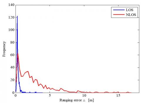
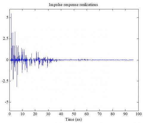
The data measured by Stefano, Wymeersch et al. are adopted for this research. These data were collected through an extensive ranging measurement campaign conducted in Massachusetts Institute of Technology (MIT), using UWB radios conforming to standards issued by the Federal Communications Commission [17-19]. The measured data shed light on how LOS and NLOS conditions affect the received waveform. Figure 1 offers a distribution histogram of ranging errors under LOS and NLOS conditions, and Figure 2 presents two typical waveforms under LOS and NLOS conditions.
Figure 1. Distribution histogram of ranging errors under LOS and NLOS conditions
Figure 2. Two typical waveforms under LOS (upper) and NLOS (lower) conditions
The following can be observed from Figures 1 and 2:
(1) The ranging errors of LOS and NLOS do not obey Gaussian distribution in the measured data. All the ranging errors are nonnegative, i.e. $\hat{d}$ (P,P1:N)³d(P,P1:N), because the first arrival path is overlooked by the leading-edge detection (LED) algorithm.
(2) The ranging errors under LOS and NLOS conditions have different properties. Under LOS condition, 98% of the measured data have a ranging error within 1m; under the NLOS, only 28% of the measured data have a ranging error within 1m.
(3) The waveforms received under LOS and NLOS conditions carry different features. These features can be used to identify NLOS waveforms and compensate for positive ranging errors through algorithms.
This section mainly introduces the principles of the three algorithms in the adaptive approach, including the MIBC, the FCE and the GPR.
3.1 The MIBC
The MIBC, proposed by Song et al. [20], provides a fast and accurate way to identify NLOS and LOS signals. This algorithm regards the NLOS identification as a classification problem with class-imbalance.
Before using the MIBC, lots of the LOS signal samples need to be processed. Here, each LOS signal sample is represented by the first two moments of their probability distribution, i.e. the mean $\bar{x}$ and covariance $\Sigma$. Then, the MIBC model was established based on the two moments and n NLOS signal samples (xi)iÎ{1,…,n}. Suppose there exists a hyperplane H(w,b) to correctly classify all the NLOS signal samples:
${{w}^{T}}{{x}_{i}}\text{-}b\ge \mathbf{0},\forall i\in \left\{ 1,...,n \right\}$ (5)
The hyperplane can also maximize the probability of correctly classifying the LOS signal samples which respect to the distribution with mean $\bar{x}$ and covariance Σ:
$\underset{\alpha ,w\ne \mathbf{0},\mathbf{b}}{\mathop{\max }}\,\alpha \underset{x\sim (\bar{x},\Sigma )}{\mathop{\inf }}\,\Pr \left\{ {{w}^{T}}x\mathbf{-}b\le 0 \right\}\ge \alpha $ (6)
where, x~($\bar{x}$, Σ) is to the class of probability distribution with mean $\bar{x}$ and covariance Σ. This hyperplane H(w,b) is the optimal solution of the following optimization problem:
$\begin{align} & \underset{w\ne \mathbf{0}}{\mathop{\min }}\,\frac{1}{2}{{w}^{T}}\Sigma w+C\sum\limits_{i=1}^{n}{{{\xi }_{i}}} \\ & s.t.{{\mathbf{(}{{x}_{i}}-\bar{x}\mathbf{)}}^{T}}w\ge 1-{{\xi }_{i}},\forall i \\ & {{\xi }_{i}}\ge 0,\forall i \\ \end{align}$ (7)
where, $C\in {{\mathbb{R}}_{+}}$ is the penalty factor to offset the model complexity and training error; ξi≥0 are the slack factors added because it is impractical to accurately classify all samples.
Considering the features of formula (4), the MIBC is actually an extension of one-class SVM [21, 22]. Of course, there are two key differences between the MIBC and the one-class SVM: First, the MIBC minimizes the Mahalanobis distance between $\bar{x}$ of the LOS signal samples and its projection on the convex hull of NLOS signal samples, instead of the l2-norm of w; Second, the MIBC separates the NLOS signal samples from the mean of the LOS signal samples, rather than from the origin of coordinates. Similar to the SVM algorithm, the solving algorithm (classifier) for the problem in formula (7) can be written as:
$f(z)=\text{sign}(\sum\limits_{i=1}^{n}{{{\alpha }_{i}}}\hat{K}(z\mathbf{,}{{x}_{i}}\mathbf{-}\bar{x})-b\ge 0)$ (8)
If the LOS and NLOS signals are not linearly separable in the original space, the nonlinear classification problem can be solved by introducing the modified kernel function $\hat{K}({{x}_{i}}\mathbf{,}{{x}_{j}})$ to map the original data to the high-dimensional space:
$\hat{K}({{x}_{i}},{{x}_{j}})=\exp (-\frac{{{({{x}_{i}}-{{x}_{j}})}^{T}}{{\Sigma }^{-1}}({{x}_{i}}-{{x}_{j}})}{{{\sigma }^{2}}})$ (9)
When it is used to identify the NLOS signals, the MIBC algorithm has an overall complexity of O(d3)+O(n3), where O(d3) is the computing load of covariance matrix, d is the dimension of signal waveform, and O(n3) is the computing load of the optimal solution to the dual problem. By contrast, the overall complexity of the SVDD is O(N 3). Because the LOS signals far outnumber the NLOS signals, the MIBC is much less complex than the SVDD.
3.2 The FCE
Some NLOS ranging errors are very large, while the others are very small. In addition, the sample distribution directly bears on the estimation of ranging errors through regression. For these two reasons, the NLOS signals can be classified according to the magnitude of NLOS ranging errors. If the ranging errors are within 1m, the NLOS signals are known as mild obstruction propagation signals; otherwise, the NLOS signals are known as severe obstruction propagation signals.
In this paper, the waveform features of these two classes of NLOS obstruction propagation signals are collected in advance, and the membership degree of each NLOS test signal belonging to mild or severe obstruction propagation signal is computed by the FCE. Based on fuzzy mathematics, the FCE can clearly and systematically quantify the membership degree of an NLOS signal in UWB positioning [23, 24].
Before using the FCE, the factor set and the determination set are set up, respectively, as:
$\left\{ \begin{align} & X=\left\{ {{x}_{\varepsilon }},{{x}_{k}},{{x}_{r}},{{x}_{m}} \right\} \\ & Y=\left\{ {{y}_{mild}},{{y}_{severe}} \right\} \\ \end{align} \right.$ (10)
where, xε, xk, xr and xm are the energy, Kurtosis, rise time and maximum amplitude of the waveform, respectively; ymild and ysevere are the two classes of obstruction propagation signals. These four factors are selected as the factor set because of the following facts: if a signal passes through severe obstruction, the energy and amplitude of the received signal will be greatly attenuated, reducing the concentration and kurtosis of the waveform amplitude distribution; it takes a longer time for the signal to rise after passing through severe obstruction than through mild obstruction. The degree of influence of each factor on judgment can be defined as:
$A=({{\eta }_{\varepsilon }},{{\eta }_{k}},{{\eta }_{r}},{{\eta }_{m}})$ (11)
Then, the two classes of obstruction propagation signals were grouped based on the principle of 10-fold cross-validation. One of the ten groups was taken as the test group, and the other nine groups were treated as training samples to provide prior values of the four factors of waveform.
The probability that an NLOS test signal x0=(ε0, k0, r0, m0) is a mild obstruction propagation signal ymild can be calculated by:
$\begin{align} & \mu _{mild}^{*}({{x}_{0}})={{\eta }_{\varepsilon }}\centerdot {{\mu }_{mild}}({{\varepsilon }_{0}})+{{\eta }_{k}}\centerdot {{\mu }_{mild}}({{k}_{0}})+ \\ & {{\eta }_{r}}\centerdot {{\mu }_{mild}}({{r}_{0}})+{{\eta }_{m}}\centerdot {{\mu }_{mild}}({{m}_{0}}) \\ \end{align}$ (12)
where, μmild(ε0), μmild(k0), μmild(r0) and μmild(m0) are the probabilities that the NLOS test signal x0 is a mild obstruction propagation signal ymild judging by one of the four factors, respectively. The specific value of μmild(ε0) can be obtained by:
$\begin{align} & {{\mu }_{mild}}({{\varepsilon }_{0}})=\frac{1}{p}\sum\limits_{j=1}^{p}{(1-\left| \frac{{{\varepsilon }_{0}}-{{\varepsilon }_{j}}}{{{\varepsilon }_{0}}} \right|)}, \\ & if\left| \frac{{{\varepsilon }_{0}}-{{\varepsilon }_{j}}}{{{\varepsilon }_{0}}} \right|>1,then\left| \frac{{{\varepsilon }_{0}}-{{\varepsilon }_{j}}}{{{\varepsilon }_{0}}} \right|=1 \\ \end{align}$ (13)
where, εj is the characteristic energy of the j-th prior waveform in the training samples of the mild obstruction propagation signals. The values of μmild(k0), μmild(r0) and μmild(m0) can be calculated in a similar manner.
Similarly, the probability $\mu _{severe}^{*}({{x}_{0}})$ that an NLOS test signal x0 is a severe obstruction propagation signal ysevere can also be obtained. Through normalization, a comprehensive evaluation result can be obtained for the NLOS test signal x0:
$\begin{align} & B=(\frac{\mu _{mild}^{*}({{x}_{0}})}{\mu },\frac{\mu _{severe}^{*}({{x}_{0}})}{\mu }), \\ & \mu =\mu _{mild}^{*}({{x}_{0}})+\mu _{severe}^{*}({{x}_{0}}) \\ \end{align}$ (14)
where, $\frac{\mu _{mild}^{*}({{x}_{0}})}{\mu }\text{and}\frac{\mu _{severe}^{*}({{x}_{0}})}{\mu }$ are the membership degrees of the mild and severe obstruction propagation signals to which the NLOS test signal x0 belongs. Here, the two membership degrees are denoted as $\omega$1 and $\omega$2, respectively. Note that if either $\omega$1 or $\omega$2 is greater than 0.7, the NLOS ranging error will directly mitigated as a single obstruction degree signal; otherwise, the estimate of the ranging error ${{\hat{\Delta }}_{i}}$ can be corrected by:
${{\hat{\Delta }}_{i}}={{\omega }_{1}}\hat{\Delta }_{i}^{mild}+{{\omega }_{2}}\hat{\Delta }_{i}^{severe}$ (15)
where, $\hat{\Delta }_{i}^{mild}$ and $\hat{\Delta }_{i}^{severe}$ are ranging errors estimated by the GPR model for mild obstruction propagation signals (M-GPR) and the GPR model for severe obstruction propagation signals (S-GPR).
The above analysis shows that the FCE outputs the membership degrees of the two classes of obstruction propagation signals to which an NLOS signal belongs, rather than directly judge which class the signal falls into.
3.3 The GPR
The Gaussian process is a desirable tool to solve regression problems [25]. The GPR model can be generally described as:
$y=f(x)+\varepsilon $ (16)
where, x is the input vector; f is the function value corresponding to the input; $\varepsilon \sim N(0,\sigma _{n}^{2})$ is a normally distributed observation noise ε; y is the observed value of each training sample. Hence, the prior distribution of the observed values of the training samples can be written as:
$y\sim N(0,K(X,X)+\sigma _{n}^{2}{{I}_{n}})$ (17)
The prior distribution of the joint probability of the observed value of a training sample and the predicted value f* of the test sample can be expressed as:
$\left[\begin{array}{c}{y} \\ {f^{*}}\end{array}\right] \sim N\left(0,\left[\begin{array}{ccc}{\boldsymbol{K}(\boldsymbol{X}, \boldsymbol{X})+\sigma_{n}^{2} \boldsymbol{I}_{n}} & {\boldsymbol{K}\left(\boldsymbol{X}, \boldsymbol{x}^{*}\right)} \\ {\boldsymbol{K}\left(\boldsymbol{x}^{*}, \boldsymbol{X}\right)} & {} & {k\left(\boldsymbol{x}^{*}, \boldsymbol{x}^{*}\right)}\end{array}\right]\right)$ (18)
where,
$\begin{aligned} \boldsymbol{K}(\boldsymbol{X}, \boldsymbol{X})=&\left[\begin{array}{ccc}{k\left(\boldsymbol{x}_{1}, \boldsymbol{x}_{2}\right)}&{k\left(\boldsymbol{x}_{1}, \boldsymbol{x}_{2}\right) \cdots} & {k\left(\boldsymbol{x}_{1}, \boldsymbol{x}_{n}\right)} \\ {k\left(\boldsymbol{x}_{2}, \boldsymbol{x}_{1}\right)} & {k\left(\boldsymbol{x}_{2}, \boldsymbol{x}_{2}\right) \cdots }&{ k\left(\boldsymbol{x}_{2}, \boldsymbol{x}_{n}\right)} \\ {\vdots} & {\vdots} & {\vdots} \\ {k\left(\boldsymbol{x}_{n}, \boldsymbol{x}_{1}\right)} & {k\left(\boldsymbol{x}_{n}, \boldsymbol{x}_{2}\right) \cdots }&{ k\left(\boldsymbol{x}_{n}, \boldsymbol{x}_{n}\right)}\end{array}\right] \\ \boldsymbol{K}\left(\boldsymbol{x}^{*}, \boldsymbol{X}\right) &=\left[k\left(\boldsymbol{x}^{*}, \boldsymbol{x}_{1}\right) k\left(\boldsymbol{x}^{*}, \boldsymbol{x}_{2}\right) \cdots k\left(\boldsymbol{x}^{*}, \boldsymbol{x}_{n}\right)\right] \end{aligned}$ (19)
Note that K(X,Y)=Kn=(kij) is an n-order Gram matrix formed by covariance of the NLOS signal training samples; kij=k(xi,xj) is the correlation between two NLOS signal training samples, xi and xj; K(K,x*)=K(x*,X)T is a pair of n-dimensional column vector and row vector formed by the covariance of an NLOS signal test sample x* and an NLOS signal training sample; k(x*,x*) is the covariance of an NLOS signal test sample.
According to the probability theory, the posterior probability distribution of the predicted value f* can be described as:
$\left. {{f}^{*}} \right|X,y,x*\sim N\left( {{{\bar{f}}}^{*}},\operatorname{cov}({{f}^{*}}) \right)$ (20)
${{\bar{f}}^{*}}=K(x*,X){{\left[ K(X,X)+\sigma _{n}^{2}{{I}_{n}} \right]}^{-1}}y$ (21)
$\begin{align} & \operatorname{cov}({{f}^{*}})=k(x*,x*)- \\ & K(x*,X)\times {{\left[ K(X,X)+\sigma _{n}^{2}{{I}_{n}} \right]}^{-1}}K(X,x*) \\ \end{align}$ (22)
${{\bar{f}}^{*}}$ and $\operatorname{cov}({{f}^{*}})$ are the mean and variance of ranging error estimate corresponding to each NLOS signal test sample x*. Here, the covariance of training samples and test samples is computed by the popular squared exponential covariance function below:
$k(x,{x}')=\sigma _{f}^{2}\exp \left[ \frac{-{{(x-{x}')}^{2}}}{2{{l}^{2}}} \right]+\sigma _{n}^{2}{{\delta }_{x,{x}'}}$ (23)
This section verifies the performance of the adaptive approach in two steps. First, the author examined the effectiveness of NLOS signal identification by the MIBC. Next, the accuracy of F-GPR in estimating the NLOS ranging errors was evaluated.
4.1 MIBC-based NLOS identification
For comparison, the MIBC and the LS-SVM were both applied to identify the NLOS signals. The identification performance was evaluated by the area under the curve (AUC): the receiver operating characteristic curve (ROC). The ratio between LOS signal training samples to NLOS signal training samples was expressed as λ=nLOS:nNLOS. In addition, the acceptance rate of the LOS signals was defined as the true rate, that is, the proportion of LOS signal samples correctly identified as LOS signals in all LOS signal samples; the acceptance rate of the NLOS signals was defined as the false positive rate, that is, the proportion of NLOS signal samples incorrectly identified as LOS signals in all NLOS signal samples. The AUC values of the two algorithms under four different λ values are listed in Table 1. The calculation times of the two algorithms under the same scenarios are compared in Table 2.
Table 1. The AUC values of the LS-SVM and the MIBC
|
λ=nLOS:nNLOS |
AUC values |
|
|
LS-SVM |
MIBC |
|
|
1:0.4 |
0.9491 |
0.9628 |
|
1:0.1 |
0.8623 |
0.9624 |
|
1:0.08 |
0.8216 |
0.9623 |
|
1:0.06 |
0.7840 |
0.9621 |
Table 2. The calculation times of the LS-SVM and the MIBC (milliseconds)
|
λ=nLOS:nNLOS |
Computational times |
Speed-up |
|
|
LS-SVM |
MIBC |
||
|
1:0.4 |
235 |
112 |
2.1 |
|
1:0.1 |
95 |
28 |
3.4 |
|
1:0.08 |
72 |
19 |
3.8 |
|
1:0.06 |
33 |
8 |
4.2 |
Figure 3. The ROCs of different algorithms at the λ of 1:0.06
As shown in Tables 1 and 2, the MIBC, which uses four waveform features in the factor set F, outperformed the LS-SVM at all four different λ values in identification accuracy and calculation efficiency.
Furthermore, the LS-SVM, the SVDD and the MIBC were simulated at the λ of 1:0.06. Their ROCs are displayed in Figure 3. Since the SVDD only uses LOS signal samples, its AUC was basically unchanged and calculation time was only half that of the LS-SVM. The MIBC had the largest AUC among the three algorithms, an evidence of its excellence in NLOS signal identification.
4.2 F-GPR-based error mitigation
In our hybrid approach, the F-GPR process basically contains the following operations: First, two GPR sub-models, M-GPR and S-GPR, were set up based on the waveform features and estimated distances $\hat{d}$ of the two classes of obstruction propagation signal training samples. Then, each test NLOS signal was subjected to the FCE, yielding two membership degrees ω1 and ω2. Meanwhile, the two GPR sub-models output two NLOS ranging error estimates $\hat{\Delta }_{i}^{mild}$ and $\hat{\Delta }_{i}^{severe}$, respectively. Next, the two estimates were weighted and added up as the final NLOS ranging error estimate ${{\hat{\Delta }}_{i}}={{\omega }_{1}}\hat{\Delta }_{i}^{mild}+{{\omega }_{2}}\hat{\Delta }_{i}^{severe}$.
In this subsection, the F-GPR is compared with the LS-SVM in the hybrid method [17], using several feature sets. The error mitigation performance was evaluated by the root mean square residual ranging error (RMS RRE): $RMSRRE=\sqrt{{1}/{N}\;\sum\nolimits_{i=1}^{N}{{{({{d}_{i}}-{{{\hat{\Delta }}}_{i}})}^{2}}}}$.
The mitigation results of the two methods on several feature set are recorded in Table 3. Besides, the cumulative distribution functions (CDFs) of the original NLOS ranging errors, those mitigated by the F-GPR and those mitigated by the LS-SVM are compared in Figure 4.
Table 3. Mitigation results of the two methods for different feature sets
|
Feature set |
Mean (m) |
RMS (m) |
||
|
F-GPR |
LS-SVM |
F-GPR |
LS-SVM |
|
|
${{F}_{1}}=\left\{ {\hat{d}} \right\}$ |
-0.0002 |
-0.0003 |
1.524 |
1.721 |
|
${{F}_{2}}=\left\{ k,\hat{d} \right\}$ |
-0.0034 |
-0.0041 |
1.358 |
1.578 |
|
${{F}_{3}}=\left\{ {{t}_{rise}},k,\hat{d} \right\}$ |
0.0004 |
0.0005 |
1.232 |
1.459 |
|
${{F}_{4}}=\left\{ {{t}_{rise}},{{\tau }_{MED}},k,\hat{d} \right\}$ |
0.0021 |
0.0027 |
1.146 |
1.432 |
|
${{F}_{5}}=\left\{ {{\varepsilon }_{r}},{{t}_{rise}},{{\tau }_{MED}},k,\hat{d} \right\}$ |
0.0106 |
0.0132 |
1.141 |
1.428 |
|
${{F}_{6}}=\left\{ {{\varepsilon }_{r}},{{t}_{rise}},{{\tau }_{MED}},{{\tau }_{RMS}},k,\hat{d} \right\}$ |
0.0145 |
0.0180 |
1.135 |
1.421 |
|
${{F}_{7}}=\left\{ {{\varepsilon }_{r}},{{r}_{\max }},{{t}_{rise}},{{\tau }_{MED}},{{\tau }_{RMS}},k,\hat{d} \right\}$ |
0.0143 |
0.0179 |
1.139 |
1.427 |
Figure 4. The CDFs of the ranging errors before and after LS-SVM and F-GPR mitigations
It can be seen from Table 3 that both methods achieved the best error mitigation effect on the feature set F6. The proposed F-GPR estimated the NLOS ranging errors more accurately than the LS-SVM. Figure 4 shows that, after mitigation by the F-GPR, the ranging errors of about 80% of the NLOS signals were within 1m, about 20% more than those mitigated by the LS-SVM. Hence, the F-GPR can effectively overcome the low estimation accuracy caused by the nonuniformity of the NLOS signal training samples.
This section attempts to make a fair comparison between our adaptive approach, the hybrid method [17], and the global GPR [19] in positioning performance. The simulation scenario was designed as follows: The tag position was defined as P=(0,0) and the NLOS conditional probability was assumed to obey 0≤PNLOS≤1; a total of N=5 reference nodes were randomly selected to identify the tag position, and each reference node i (1≤i≤N) randomly extracts a received signal waveform from the measured data, which contains PNLOS waveforms of the NLOS signals and 1-PNLOS waveforms of the LOS signals. Then, the position Pi of each reference node i (1≤i≤N) can be calculated by:
${{P}_{i}}={{d}_{i}}(P,{{P}_{i}})(\sin (2\pi ({i-1}/{N}\;)),\cos (2\pi ({i-1}/{N}\;)))$ (24)
where, di(P,Pi) is the real distance between the reference node and the tag.
After extracting the waveforms and obtaining the estimated distances ${{\hat{d}}_{i}}\left( P,{{P}_{i}} \right)$, the adaptive approach, the hybrid method and the global GPR were separately applied to mitigate NLOS ranging errors. Finally, the tag position was estimated by l1-norm and l2-norm minimization [12]:
$\hat{P}=\underset{P}{\mathop{\arg \min }}\,{{\left\| l\left( P,{{P}_{1:N}} \right)-y \right\|}_{\alpha }}$ (25)
where, $\alpha \in \left\{ 1,2 \right\}$,
$l\left( P,{{P}_{1:N}} \right)=\left[ {{l}_{1}}(P,{{P}_{1}}),\cdots ,{{l}_{N}}(P,{{P}_{1}}) \right]$ (26)
${{l}_{i}}(P,{{P}_{i}})=\log \left( {{{\hat{d}}}_{i}}\left( P,{{P}_{i}} \right)-{{d}_{i}}\left( P,{{P}_{i}} \right) \right)$ (27)
$y=\left[ \log ({{{\hat{\Delta }}}_{1}}),\cdots \log ({{{\hat{\Delta }}}_{N}}) \right]$ (28)
The positioning accuracy of each algorithm was evaluated by the outage probability:
${{p}_{out}}({{e}_{th}})=pro\left\{ \left\| P-\hat{P} \right\|>{{e}_{th}} \right\}$ (29)
where, eth is the preset allowable error; $\left\| P-\hat{P} \right\|$ is the position error. Under each NLOS conditional probability, an outage occurs if $\left\| P-\hat{P} \right\|$ exceeds eth. The three algorithms were tested under four scenes: changing allowable error under the NLOS conditional probability of 0.2, changing allowable error under the NLOS conditional probability of 0.8, changing NLOS conditional probabilities under the allowable error of 0.5m, and changing NLOS conditional probabilities under the allowable error of 2m. For each scene, the outage probability was determined through 5,000 Monte-Carlo simulations.
5.1 Simulation 1 (outage probabilities at different allowable errors)
Figures 5 and 6 show the outage probability curves of the three algorithms under PNLOS=0.2 and PNLOS=0.8, respectively.
As shown in Figure 5, under the same allowable error ${{e}_{th}}$, the outage probability of global GPR method was greater than that of hybrid method or adaptive approach, whether the tag position was estimated by l1-norm or l2-norm minimization. The reason for the high outage probability is as follows: global GPR makes use of all the estimated distances in positioning; however, the estimated distances under mitigated NLOS are not so accurate as the estimated distances under the LOS; the positioning based on these estimated distances will face a high redundant error.
It can also be seen that the adaptive approach achieved a lower outage probability than the hybrid method. This is because the adaptive approach has better identification probability for the NLOS signals, although both methods only rely on the estimated distances under the LOS for positioning.
In addition, under PNLOS=0.2, all three methods performed better when the tag position was estimated based on l2-norm than l1-norm. A possible reason is that, under l1-norm minimization, some components of the ranging error vector ${{\hat{d}}_{i}}\left( P,{{P}_{i}} \right)-{{d}_{i}}\left( P,{{P}_{i}} \right)$ are adjusted to zero to find sparse solution, which pushes up the error of the remaining components.
As shown in Figure 6, under the same allowable error eth, the adaptive approach realized a smaller outage probability than global GPR and hybrid method, whether the tag position was estimated by l1-norm or l2-norm minimization. This means the LS-SVM in the hybrid method leads to a higher outage probability than the F-GPR of the adaptive approach. The result can be attributed to two reasons. First, the hybrid method is outshined by the adaptive approach in identification performance, though both classifies NLOS signals and LOS signals in advance. Second, the LS-SVM in the hybrid method establishes the regression model directly, without considering the suppression of the nonuniform distribution of NLOS signal samples on the regression effect, while the F-GPR fully recognizes the nonuniform distribution and divides the samples into mild and severe obstruction propagation signals.
Figure 5. Outage probabilities of the three algorithms at PNLOS=0.2
Figure 6. Outage probabilities of the three algorithms at PNLOS=0.8
5.2 Simulation 2 (outage probabilities at different NLOS conditional probabilities)
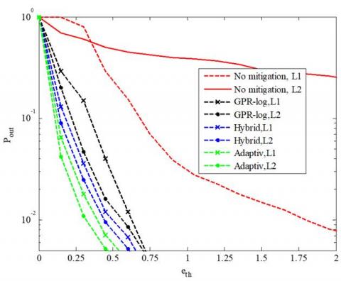
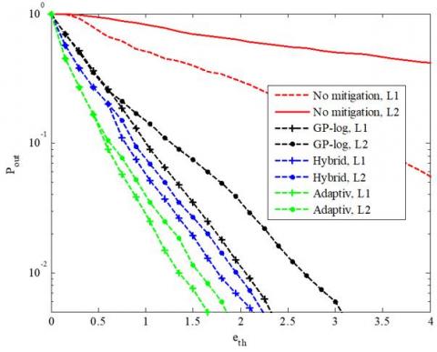
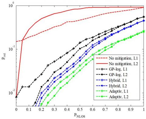
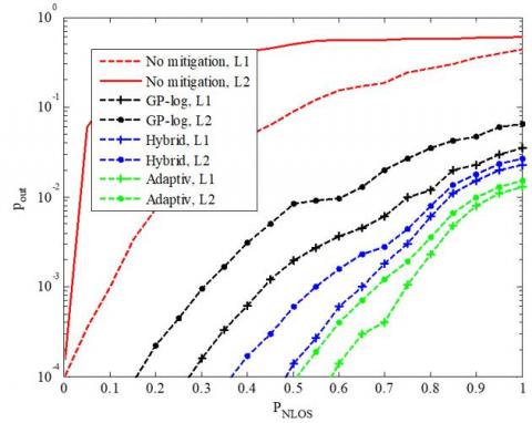
Figures 7 and 8 show the outage probability curves of the three algorithms under eth=0.5m and eth=2m, respectively.
As shown in Figure 7, under the same NLOS conditional probability, the outage probability of global GPR method was greater than that of hybrid method or adaptive approach, whether the tag position was estimated by l1-norm or l2-norm minimization. There are two causes of this situation. First, the global GPR does not discriminate the NLOS signals from the LOS signals, but directly set up the regression model. The model cannot make accurate estimations due to the uneven distribution of training samples. That is why the global GPR performed poorly in estimation of ranging errors and tag positioning. Second, the estimated distances under the NLOS are used, although those under the LOS are sufficient for positioning, leading to redundant errors.
Figure 7. Outage probabilities of the three algorithms at eth=0.5m
Figure 8. Outage probabilities of the three algorithms at eth=2m
Furthermore, the hybrid method had a higher outage probability than our adaptive approach, because the LS-SVM is less precise than the F-GPR. The LS-SVM’s lag in precision is resulted from its relatively poor identification performance, and the failure to divide nonuniform NLOS signals into mild and severe obstruction propagation signals.
As shown in Figure 8, the outage probabilities of all three algorithms at eth=2m were lower than those at eth=0.5m. Under the same NLOS conditional probability, the adaptive approach boasted the lowest outage probability, whether the tag position was estimated by l1-norm or l2-norm minimization. Meanwhile, l1-norm minimization achieved the better positioning result, owing to its high robustness.
In real-world scenarios, the UWB positioning is confronted with serious positioning error under the presence of the NLOS signals. The existing methods to mitigate the error all have certain problems or limitations. To solve the problems, this paper proposes an adaptive approach for UWB positioning in complex environment based on machine learning. The adaptive approach integrates the MIBC with the F-GPR to achieve accurate and flexible positioning with a limited computing load. The excellence of the proposed adaptive approach was fully proved through simulations, in comparison with the hybrid method and the global GPR.
[1] Güvenç, I., Chong, C.C., Watanabe, F., Inamura, H. (2007). NLOS identification and weighted least-squares localization for UWB systems using multipath channel statistics. EURASIP Journal on Advances in Signal Processing, 2008(1): 1-14. https://doi.org/10.1155/2008/271984
[2] Dabove, P., Di Pietra, V., Piras, M., Jabbar, A.A., Kazim, S.A. (2018). Indoor positioning using Ultra-wide band (UWB) technologies: Positioning accuracies and sensors' performances. In 2018 IEEE/ION Position, Location and Navigation Symposium (PLANS): 175-184. https://doi.org/10.1109/PLANS.2018.8373379
[3] Sharma, P., Vaish, A., Yaduvanshi, R.S. (2019). The design of a turtle-shaped dielectric resonator antenna for ultrawide-band applications. Journal of Computational Electronics, 18(4): 1333-1341. https://doi.org/10.1007/s10825-019-01374-8
[4] Xu, Y., Shmaliy, Y.S., Li, Y.Y., Chen, X.Y. (2017). UWB-based indoor human localization with time-delayed data using EFIR filtering. IEEE Access, 5: 16676-16683. https://doi.org/10.1109/ACCESS.2017.2743213
[5] Xu, Y., Shen, T., Chen, X.Y., Bu, L.L., Feng, N. (2019). Predictive adaptive Kalman filter and its application to INS/UWB-integrated human localization with missing UWB-based measurements. International Journal of Automation and Computing, 16(5): 604-613. https://doi.org/10.1007/s11633-018-1157-4
[6] Ke, W., Wu, L.N. (2011). Mobile location with NLOS identification and mitigation based on modified Kalman filtering. Sensors, 11(2): 1641-1656. https://doi.org/10.3390/s110201641
[7] Sun, F., Yin, H.R., Wang, W.D. (2011). Finite-resolution digital receiver for UWB TOA estimation. IEEE Communications Letters, 16(1): 76-79. https://doi.org/10.1109/lcomm.2011.111611.112074
[8] Kok, M., Hol, J.D., Schön, T.B. (2015). Indoor positioning using ultrawideband and inertial measurements. IEEE Transactions on Vehicular Technology, 64(4): 1293-1303. https://doi.org/10.1109/TVT.2015.2396640
[9] Canepa, A., Talebpour, Z., Martinoli, A. (2017). Automatic calibration of ultra wide band tracking systems using a mobile robot: A person localization case-study. In 2017 International Conference on Indoor Positioning and Indoor Navigation (IPIN), 1-8. https://doi.org/10.1109/IPIN.2017.8115905
[10] Huang, S.H., Guo, Y., Zha, S.S., Wang, F.L., Fang, W.G. (2017). A real-time location system based on RFID and UWB for digital manufacturing workshop. Procedia Cirp, 63: 132-137. https://doi.org/10.1016/j.procir.2017.03.085
[11] Cai, X.F., Ye, L., Zhang, Q. (2018). Ensemble learning particle swarm optimization for real-time UWB indoor localization. EURASIP Journal on Wireless Communications and Networking, 2018(1): 125-139. https://doi.org/10.1186/s13638-018-1135-0
[12] Yang, X.F. (2018). NLOS mitigation for UWB localization based on sparse pseudo-input Gaussian process. IEEE Sensors Journal, 18(10): 4311-4316. https://doi.org/10.1109/JSEN.2018.2818158
[13] Yang, X.F., Zhao, F., Chen, T.J. (2018). NLOS identification for UWB localization based on import vector machine. AEU-International Journal of Electronics and Communications, 87: 128-133. https://doi.org/10.1016/j.aeue.2018.02.003
[14] Shi, Q., Zhao, S.H., Cui, X.W., Lu, M.Q., Jia, M.D. (2019). Anchor self-localization algorithm based on UWB ranging and inertial measurements. Tsinghua Science and Technology, 24(6): 728-737. https://doi.org/10.26599/TST.2018.9010102
[15] Yu, K.G., Wen, K., Li, Y.B., Zhang, S., Zhang, K.F. (2018). A novel NLOS mitigation algorithm for UWB localization in harsh indoor environments. IEEE Transactions on Vehicular Technology, 68(1): 686-699. https://doi.org/10.1109/TVT.2018.2883810
[16] Wen, K., Yu, K., Li, Y.B. (2017). NLOS identification and compensation for UWB ranging based on obstruction classification. In 2017 25th European Signal Processing Conference (EUSIPCO), 2704-2708. https://doi.org/10.23919/EUSIPCO.2017.8081702
[17] Marano, S., Gifford, W.M., Wymeersch, H., Win, M.Z. (2010). NLOS identification and mitigation for localization based on UWB experimental data. IEEE Journal on Selected Areas in Communications, 28(7): 1026-1035. https://doi.org/10.1109/JSAC.2010.100907
[18] Tian, S.W., Zhao, L.W., Li, G.X. (2014). A support vector data description approach to NLOS identification in UWB positioning. Mathematical Problems in Engineering, 1-6. http://dx.doi.org/10.1155/2014/963418
[19] Wymeersch, H., Maranò, S., Gifford, W.M., Win, M.Z. (2012). A machine learning approach to ranging error mitigation for UWB localization. IEEE Transactions on Communications, 60(6): 1719-1728. http://dx.doi.org/10.1109/TCOMM.2012.042712.110035
[20] Song, B., Li, S.L., Tan, M., Ren, Q.H. (2018). A fast imbalanced binary classification approach to NLOS identification in UWB positioning. Mathematical Problems in Engineering, 1-8. https://doi.org/10.1155/2018/1580147
[21] Suykens, J.A.K., Vandewalle, J. (1999). Least squares support vector machine classifiers. Neural Processing Letters, 9(3): 293-300. https://doi.org/10.1023/A:1018628609742
[22] Choi, Y.S. (2009). Least squares one-class support vector machine. Pattern Recognition Letters, 30(13): 1236-1240. https://doi.org/10.1016/j.patrec.2009.05.007
[23] Zadeh, L.A. (1965). Fuzzy sets. Information and Control, 8(3): 338-353. https://doi.org/10.1016/S0019-9958(65)90241-X
[24] Dubois, D., Prade, H. (1982). Towards fuzzy differential calculus part 1: Integration of fuzzy mappings. Fuzzy sets and Systems, 8(1): 1-17. https://doi.org/10.1016/0165-0114(82)90025-2
[25] Park, C., Huang, J.Z., Ding, Y. (2011). Domain decomposition approach for fast Gaussian process regression of large spatial data sets. Journal of Machine Learning Research, 12(4): 1697-1728. https://doi.org/10.1016/j.neunet.2010.12.008