Weixing Hua | Weiming Zhang | Jiang Li* | Xuexin Li | Xiang Li | Tingao Shen
OPEN ACCESS
This paper attempts to measure the jet flow field of different nozzles accurately, and optimize the effect of the jetting devices. For this purpose, four nozzles with different structures were physically and mathematically modelled, including conical-cylindrical nozzle, conical nozzle, cylindrical nozzle and streamlined nozzle. The turbulence was described by the improved standard k-epsilon (k-ε) turbulence model. Then, the measurement space was meshed into unstructured triangular grids, with high grid density in key areas. Next, the flow field inside and outside each nozzle was simulated on ANSYS Fluent, and the jet velocity field distribution at different positions, velocity fields and kinetic turbulence were analyzed based on the simulation results. The analysis shows that the streamlined nozzle achieved the highest flow velocity and lowest turbulent energy at the centerline of the flow field, and should be prioritized in actual applications. The conical-cylindrical nozzle strikes a good balance between efficiency and cost, providing a good option for jetting operations. By contrast, conical nozzle and cylindrical nozzle should not be adopted. The cylindrical segment can stabilize the shape of the jet by increasing the jet acceleration and peak velocity. The nozzle structure should be optimized to reduce the energy loss in each phase of energy conversion, thereby lowering the energy required to destroy a unit volume of the target. The simulation results shed important new light on the selection of nozzle for jetting devices.
flow field, specific energy, impact distance, nozzle structure
The jetting devices have been widely used in cutting, cleaning, fine processing and medical fields [1, 2]. The jet performance depends on many components, especially the nozzle. For example, the impact effect and divergence of the jet are affected by the velocity and turbulence in the axial direction. Therefore, the parameters of the flow field inside nozzles of varied structures must be measured accurately, before the design of jetting devices [3-5]. However, the jetting devices often operate in extreme conditions, including high jet pressure, high velocity and severe turbulence. Under these conditions, it is difficult to measure the waterjet flow field accurately by traditional methods. Currently, nozzle performance is mainly evaluated by comparing its cutting depth through experiments. But this approach cannot measure the flow field parameters directly.
Many scholars have explored the relationship between jet and nozzle, aiming to optimize the nozzle structure and improve jetting performance. For example, Zeidan et al. [6] and Ahmed et al. [7] investigate the nozzle force and other nozzle parameters in the jet system. Nie et al. [8] and Pozzetti and Peters [9] probe deep into the reverse thrust of jet, and examine the thrust coefficient and pressure distribution on the inner wall of the nozzle, revealing the significant impacts of nozzle diameter and inlet/outlet conditions on reverse thrust. Li et al. [10] found that conical nozzle has a larger reverse thrust than cylindrical nozzle, under the same conditions. Akihisa et al. [11] simulated the reverse thrust of jet and then optimized the nozzle. Barsukov et al. and Mieszala et al. [12, 13] conducted simulation and experiment on the reverse thrust of the two-phase jet of conical nozzle, concluding that the two-phase jet can greatly bolster the reverse thrust.
In the field of jet cutting, the research focus lies in how jet features and cutting performance are influenced by the parameters and position of nozzle [14-16]. For instance, Eckart Uhlmann et al. [17] discovered that jet velocity peaked at the cone angle of 400. Ozcelik et al. [18] studied the impacts of cone angle on surface roughness of the stone after jetting, pointing out that the surface roughness is large at a small or large cone angle and small at a medium cone angle. Wang [19] explored the effects of nozzle position on coating removal efficiency, and learned that the peak efficiency is achieved when the nozzle-target distance is shorter than 500mm.
Despite the above studies, there is little report on the complex relationship between the energy loss, nozzle parameters and inlet/outlet conditions [20, 21]. Being the load in the jet system, the nozzle converts the pressure energy of water into kinetic energy, creating a jet that acts on external target. It is inevitable for the conversion process to have some energy loss. The size of the loss directly depends on the nozzle parameters and inlet/outlet conditions. The energy loss not only affects the jetting efficiency, but also harms the operator and system stability, for the lost energy exists as heat and sound energy. Therefore, an important aspect of optimizing nozzle structure and jetting efficiency is to disclose the relationship between energy loss and nozzle parameters [22-25].
In this paper, four nozzles with different structures, namely, conical-cylindrical nozzle, conical nozzle, cylindrical nozzle and streamlined nozzle, were physically and mathematically modelled. Then, the flow field inside and outside each nozzle was simulated on ANSYS Fluent. The simulation results shed important new light on the selection of nozzle for jetting devices.
2.1 Physical models of nozzles with different structures
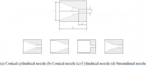
According to the common classification of nozzles in jetting devices, the physical models of four basic nozzle structures were established, including conical-cylindrical nozzle, conical nozzle, cylindrical nozzle and streamlined nozzle. The physical models are presented in Figure 1. The dimensions of the four nozzles are listed in Table 1.
Figure 1. Physical models of the four nozzles
Table 1. Dimensions of the four nozzles
|
No. |
Type |
Total length L (mm) |
Cylindrical segment length L1(mm) |
Outer diameter D(mm) |
Inner diameter d (mm) |
Conical angle α(°) |
|
1 |
Cone cylinder |
20 |
5 |
3 |
1 |
22.6 |
|
2 |
Cone |
20 |
0 |
3 |
1 |
22.6 |
|
3 |
Cylindrical |
20 |
5 |
3 |
1 |
/ |
|
4 |
Streamlined |
20 |
5 |
3 |
1 |
/ |
2.2 Selection of nozzle-target distance
The impact force of the jet reaches the maximum when the nozzle is at a certain distance from the target. Further increase in that distance will reduce the impact force. Normally, the nozzle-target distance is 100~300 times the nozzle diameter. The attenuation of the impact force with nozzle-target distance can be empirically defined as:
$\mathrm{p}_{i m}=389 \cdot e^{-0.0165 \cdot s}$ (1)
where, pim is the impact force of the jet (MPa); s is the nozzle-target distance (mm). For comparison, the nozzle-target distances of different nozzles were all set to 40mm, which falls within the effective target range of the maximum impact force.
3.1 Turbulence model
Considering the features of the jet flow field, the standard k-epsilon (k-ε) turbulence model was selected for numerical simulation:
For turbulent kinetic energy:
$\frac{\partial(\rho k)}{\partial t}+\frac{\partial\left(\rho u_{i} k\right)}{\partial x_{i}}=\frac{\partial}{\partial x_{j}}\left[\left(\mu+\frac{\mu_{\tau}}{\sigma_{k}}\right) \frac{\partial k}{\partial x_{j}}\right]+G_{k}+G_{b}-\rho \varepsilon-Y_{M}+S_{k}$ (2)
For dissipation:
$\frac{\partial (\rho \varepsilon )}{\partial t}+\frac{\partial (\rho {{u}_{i}}\varepsilon )}{\partial {{x}_{i}}}=\frac{\partial }{\partial {{x}_{j}}}\left[ \left( \mu +\frac{{{\mu }_{\tau }}}{{{\sigma }_{\varepsilon }}} \right)\frac{\partial \varepsilon }{\partial {{x}_{j}}} \right]+{{C}_{1\varepsilon }}\frac{\varepsilon }{k}({{G}_{k}}-{{C}_{3\varepsilon }}{{G}_{b}})-{{C}_{2\varepsilon }}\rho \frac{{{\varepsilon }^{2}}}{k}+{{S}_{\varepsilon }}$ (3)
where, Gk is the turbulent flow energy produced by velocity gradient; Gb is the buoyancy energy generated by buoyancy; YM is the dissipation fluctuations in the compressible turbulence; C1e, C2e and C3e are empirical constants; sk and se are Prandtl numbers; Sk and Se are user-defined source terms.
The k-ε turbulence model works effectively in areas with good turbulent development. However, the turbulence is not fully developed in the near-wall region inside the jet nozzle. This region is dominated by the influence of molecular viscosity, especially right next to the wall. The flow may be laminar at the bottom layer. Hence, the k-ε turbulence model cannot be directly applied in the near-wall region.
To solve this problem, the near-wall region was not solved directly but derived from the variables of the core area of the turbulence by semi-empirical formulas. The control volume adjacent to the wall was directly obtained by functional relationship. Then, the turbulent energy generating terms in the control volume that that constitutes the source terms of the formula, namely, Gk and e can be computed based on the local equilibrium assumption:
$\mathrm{G}_{k}=\tau_{w} \frac{\partial u}{\partial y}=\tau_{w} \frac{\tau_{w}}{\kappa \rho C_{\mu}^{1 / 4} k_{p}^{1 / 2} \Delta y_{p}}$ (4)
$\varepsilon=\frac{C_{\mu}^{3 / 4} k_{p}^{3 / 2}}{\kappa \Delta y_{p}}$ (5)
Then, the dissipation rate in the control volume can be determined by formula (5). In this way, the flow of the near-wall region can be effectively obtained in an efficient manner.
3.2 Jet energy loss model
The jetting devices convert electrical or chemical energy into mechanical energy, which acts on the target in the form of jet energy. The nozzle plays a critical role in the conversion of mechanical energy to jet energy. To measure the conversion efficiency, the concept of specific energy was introduced: the energy required to destroy per unit volume of the target. Then, the energy loss can be computed based on the efficiency of specific efficiency:
$E=P / V$ (6)
where, P is the jet energy; V is the target damage per unit time. The value of V depends on the cutting depth and width as well as the relative cutting velocity. The relative cutting velocity v can be obtained by:
$v=h w m$ (7)
where, h is the cutting depth; w is the cutting width; m is the cutting length per unit of time.
Before it reaches the nozzle, the high-pressure water has already lost half of its energy due to hydraulic friction in the pumping and transmission process. Therefore, the nozzle’s diameter and flow coefficient must be optimized to improve the energy efficiency. Here, the jet pressure at all nozzles is set to 50MPa, according to the pressure setting of abrasive jet machining. Actual measurements show that the energy that destroys the target is only about 1/8 of the total energy. This calls for efficient use of jet energy in high-pressure jetting devices. The key lies in the optimization of nozzle structure.
4.1 Meshing
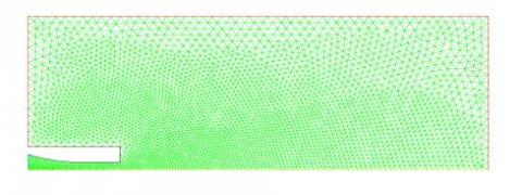
Figure 2. Grids of the flow field of conical nozzle
The flow field inside and outside the nozzle was meshed by a meshing software. As shown in Figure 2, the conical nozzle is taken as the example to explain the meshing process. Considering its symmetry, only the half of the flow field was meshed into unstructured triangular grids. The grid density was higher at the key positions inside the nozzle.
4.2 Boundary conditions
The nozzle inlet was simulated as a pressure boundary (50MPa), the nozzle wall as ano-slip adiabatic boundary, the outlet as a free outflow boundary, the lower edge as a symmetry boundary, and the other edges as pressure outlet boundaries. The temperature was set to normal temperature.
4.3 Unstructured grid computation
As mentioned above, some parts of the nozzle were meshed into denser grids to reflect the relatively large variation of the flow field, and the entire flow field was simulated as unstructured grids. Unlike structured grids, unstructured grids do not follow any fixed law of grid and node arrangement. The type, shape and size of the grids may vary throughout the computation, making it difficult to simulate the flow field. Hence, the flow field algorithm based on the unstructured grids was improved as follows.
In general form, the discrete governing formula can be expressed as:
$\frac{\partial (\rho \varphi )}{\partial t}+\text{div}(\rho u\phi )=\text{div}(\Gamma \text{grad}\phi )+S$ (8)
This conservation-type formula can integrate the time domain and the control volume. For any control volume, the P integral can be obtained as:
$\int_{\Delta V}{\frac{\partial (\rho \varphi )}{\partial t}\text{d}V}+\int_{\Delta V}{\text{div}(\rho u\phi )\text{d}V}=\int_{\Delta V}{\text{div}(\Gamma \text{grad}\phi )\text{d}V}+\int_{\Delta V}{S\text{d}V}$ (9)
Then, the divergence theorem was introduced to obtain the volume fraction of the convection term and the diffusion term in the above formula:
$\int_{\Delta V}{\text{div}(a)\text{d}V}\text{=}\int_{\Delta S}{\upsilon \cdot a\text{d}S}=\int_{\Delta S}{{{\upsilon }_{i}}\cdot {{a}_{i}}\text{d}S}=\int_{\Delta S}{({{a}_{x}}\cdot {{\upsilon }_{x}}+{{a}_{y}}\cdot {{\upsilon }_{y}}+{{a}_{z}}\cdot {{\upsilon }_{z})}\text{d}S}$ (10)
where, $\Delta $V is the 3D integral domain; $\Delta $S is the closed transition interface; $a$ is a random vector; $\upsilon$ is the unit normal vector of a surface. The tensors in the above formula are of the same size. Substituting formula (10) into formula (8), we have:
$\int_{\Delta V}{\frac{\partial (\rho \varphi )}{\partial t}\text{d}V}+\int_{\Delta S}{\rho \phi {{u}_{i}}{{\upsilon }_{i}}\text{d}S}=\int_{\Delta S}{\Gamma \frac{\partial \phi }{\partial {{x}_{i}}}{{\upsilon }_{i}}\text{d}S}+\int_{\Delta V}{S\text{d}V}$ (11)
where, vi is the unit normal vector one each surface; ui is the velocity component. The transient term in formula (11) can be described as:
$\int_{\Delta V}{\frac{\partial (\rho \varphi )}{\partial t}\text{d}V}=\frac{{{(\rho \phi )}_{P}}-(\rho \phi )_{P}^{0}}{\Delta t}\Delta V$ (12)
where, 0 denotes is value of the previous time step; $\Delta $t is time step; fp is the P value at the center of the control volume.
The source term and diffusion term of formula (11) can be respectively depicted as:
$\int_{\Delta V}{S\text{d}V}=S\Delta V=({{S}_{C}}+{{S}_{P}}{{\phi }_{P}})\Delta V={{S}_{C}}\Delta V+{{S}_{P}}{{\phi }_{P}}\Delta V$ (13)
$\int_{\Delta S}{\Gamma \frac{\partial \phi }{\partial {{x}_{i}}}{{\upsilon }_{i}}\text{d}S}={{\sum\limits_{E=1}^{{{N}_{S}}}{\left\{ \left( {{\phi }_{E}}-{{\phi }_{P}} \right)/\sqrt{\delta {{x}^{2}}+\delta {{y}^{2}}}\cdot \left[ \Gamma \left( {{\upsilon }_{x}}\Delta y-{{\upsilon }_{y}}\Delta x \right) \right] \right\}}}_{E}}+{{C}_{diff}}$ (14)
where, Ns is the total number of surfaces of control volume P; E is the volume of each control body having a common interface with control volume P; vx and vy are the unit normal vector of the interface; $\delta $x and $\delta $y are the vector components of node P to node E between the two control volumes; Cdiff is the intersection on the common interface.
The convection term of formula (11) can be defined as:
$\int_{\Delta S}{\rho \phi {{u}_{i}}{{\upsilon }_{i}}\text{d}S}=\sum\limits_{E=1}^{{{N}_{S}}}{{{\left[ \rho \phi \left( u\Delta y-v\Delta x \right) \right]}_{E}}}$ (15)
where, $\phi$ is the stream term of the interface in the low-order discrete format. The value of $\phi$ can be obtained by interpolation.
Substituting formulas (12)-(15) into formula (11), the discrete formulas can be obtained based on unstructured grids through the integration of the time domain:
${{a}_{P}}{{\phi }_{P}}=\sum\limits_{E}^{{{N}_{S}}}{{{a}_{E}}{{\phi }_{E}}+{{b}_{P}}}$ (16)
where, ap and bp are two coefficients:
${{a}_{P}}=\sum\limits_{E}^{{{N}_{S}}}{{{a}_{E}}+\frac{{{({{\rho }_{P}}\Delta V)}^{0}}}{\Delta t}-{{S}_{P}}\Delta V}$ (17)
${{b}_{P}}=\frac{{{({{\rho }_{P}}{{\phi }_{P}}\Delta V)}^{0}}}{\Delta t}+{{S}_{C}}\Delta V$ (18)
The size of ap depends on the discrete format of the stream term. The discrete form of the momentum, velocity and pressure correction formulas was derived in a similar way, laying the basis for numerical simulation.
5.1 Jet velocity field distribution at different positions
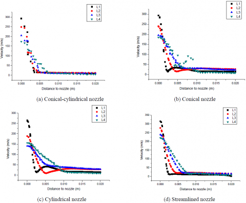
Four positions were selected at 10, 20, 30 and 40mm away from the nozzle, respectively. Then, the lines passing the four positions, which are vertical to the symmetrical axis of the nozzle, were drawn. The flow field data on the four lines were recorded for each of the four nozzles (namely, conical-cylindrical nozzle, conical nozzle, cylindrical nozzle and streamlined nozzle). The velocity profiles of the four nozzles are displayed in Figure 3.
Figure 3. The velocity profiles of the four nozzles
As shown in Figure 3, whichever the nozzle, the jet flow field velocity always declined gradually along the vertical direction of the symmetrical axis and finally reached the minimum level. The velocity varied from place to place. On line L1, which is the closest to the nozzle, the velocity distribution was sharper than that of any other line and the velocity peaked on the symmetrical axis.
The streamlined nozzle had the fastest velocity (315m/s), while the other three nozzles failed to reach 300m/s. The peak velocity of the cylindrical nozzle was only 264m/s, about 15% lower than the velocity of the streamlined nozzle under the same pressure. The low velocity greatly reduces the jetting efficiency.
For the conical-cylindrical nozzle, the flow field velocity distribution was quite messy. The velocities on all four lines were basically the same, starting with 0.015maway from the symmetrical axis.
For the conical nozzle, the flow field velocity distribution was rather obvious, with was a sudden velocity increase on line L4, the farthest line from the nozzle.
For the cylindrical nozzle, the flow field velocity distribution had two valleys, rather than a balanced tail. The minimum velocities on L1 and L4 were smaller than those of L2 and L3.
For the streamlined nozzle, the flow field velocity changed more gradual than that of any other nozzle. With the increase in the distance to the nozzle, the velocities at different positions evenly decreased to the minimum levels.
The above analysis shows that various nozzle structures differ greatly in velocity distribution. Next, the flow fields of different nozzles are compared in details.
5.2 Analysis of velocity field
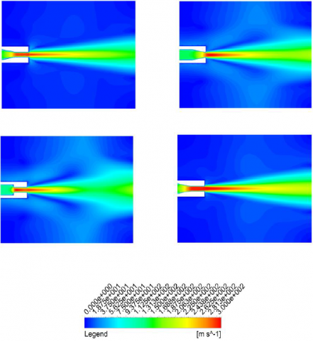
The ANSYS Fluent was adopted to simulate the four nozzles under the abovementioned boundary conditions. The water was pumped into the nozzle via the left inlet by a high-pressure pump. Then, the water flow was densified and accelerated through the nozzle, and emitted from the outlet as a high-pressure jet. Because the water is much denser than the air, the effects of the air on the fluid in the nozzle were neglected. The velocity cloud maps of the four nozzles are presented in Figure 4.
Figure 4. Velocity cloud maps of the four nozzles
Figure 4 shows great differences between the four nozzles in flow field. In conical nozzle, the velocity increased from the left to the right of the cylindrical segment, and then gradually decreased. The velocity in this nozzle was slower than that of the streamlined nozzle, but faster than the conical-cylindrical and cylindrical nozzles.
The holding time of the peak velocity has a positive impact on impact effect and specific energy efficiency. For the conical nozzle, the peak velocity appeared at the nozzle outlet, unlike any of the other nozzles. This is because the conical nozzle has no cylindrical segment. The water accelerated by the nozzle is directly jetted out, rather than form a stable flow field.
Moreover, the conical nozzle had a shorter impact distance than conical-cylindrical and streamlined nozzles, indicating that the cylindrical segment can enhance the impact effect and reduce the specific energy loss.
The cylindrical nozzle is easy to fabricate and install, and has been widely adopted in early jetting devices. However, the simulation results show that the cylindrical segment had a great impact on the flow velocity and impact distance, due to the suddenly narrowed flow path: the cylindrical nozzle achieved the shortest impact distance among all four nozzles. Hence, this type of nozzle should not be adopted in actual practice.
The streamlined nozzle realized the fastest velocity and fastest impact distance, an evidence of excellent impact effect. The results demonstrate the suitability of this nozzle for jet cutting and finishing. Nonetheless, this nozzle has not been extensively applied. Thus, the streamline nozzle structure should be considered to enhance the jetting effect.
In Figure 4, the red area represents the high-velocity area in the flow field. The length and position of this area reflect the acceleration performance of the corresponding nozzle. It can be seen that, the streamlined nozzle boasted the best acceleration effect, followed by the conical-cylindrical nozzle and the conical nozzle. The cylindrical nozzle was the poorest in acceleration. These results can be explained as follows: In the streamlined nozzle, the fluid flow lines are relatively uniform and the velocity loss is rather limited. By contrast, in the cylindrical nozzle, the flow field changes abruptly in the acceleration process, and the velocity is slowed down. Thus, the jet velocity and impact force both decreased.
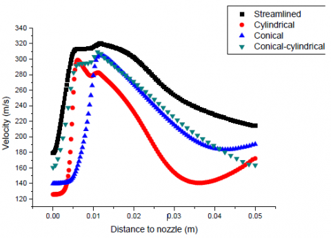
To sum up, the four nozzles have different jetting effects in different situations. Considering the velocity cloud maps, the velocities at the center of the symmetrical axis of the flow field of the four nozzles were compared in Figure 5.
It can be seen from Figure 5 that the streamlined nozzle brought the fastest velocity among the four nozzles, and its velocity peaked at 320m/s. In addition, this nozzle also enjoyed the longest impact distance, about 0.02m away from the nozzle outlet. This means the streamlined structure can improve the jet flow field and jetting efficiency. The conical-cylindrical nozzle had the second-best peak velocity and impact distance among the four nozzles. Due to the lack of a cylindrical segment, the velocity of the conical nozzle plunged deeply after reaching the peak of 300m/s. Besides, the conical nozzle failed to maintain a stable impact distance, which limits its application potential. As for the cylindrical nozzle, the peak velocity appeared within the nozzle. Although it was not very small, the velocity gradually declined after leaving the nozzle. The cylindrical nozzle had the smallest velocity and most unstable impact distance among all four nozzles.
Figure 5. Flow field center velocities of the four nozzles
5.3 Analysis of kinetic turbulence
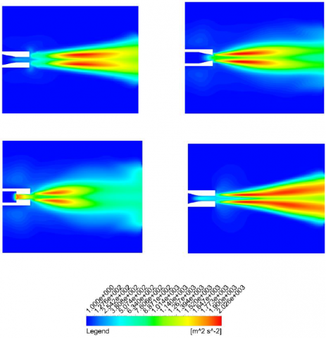
Since the water jet is a fully developed turbulence, the energy consumption is closely correlated with the turbulent energy during the injection process. Thus, the k-ε turbulence model was selected to simulate the four nozzles. The cloud maps of turbulent energy are presented in Figure 6.
Figure 6. Cloud maps of turbulent energy of the four nozzles
As shown in Figure 6, turbulent energy of the conical-cylindrical nozzle started to develop from both sides of the outlet, and gradually expanded to the middle. The energy acted on the fluids on both sides, and peaked at the middle. With the growth of the turbulent energy, its scope of influence gradually widened, and finally reached the outlet wall. The core area of the turbulent energy was shaped like a shuttle, indicating that the energy generated by the jet was mostly consumed at the center. This finding makes it easy to judge the energy conversion degree of the jet.
The turbulent energy of the conical nozzle increased from the right side within the nozzle, and peaked on both sides of the fluid center. Compared with the conical-cylindrical nozzle, the peak energy of conical nozzle spanned for a short distance and close to the nozzle. This means intense energy conversion occurs at the outlet of conical nozzle, creating a high turbulence that reduces the jet density. There are two possible causes to this phenomenon: First, the flow continues to accelerate from the original angle after being ejected from the conical nozzle, which reduces the jet intensity; Second, the excessively high Reynolds number at the outlet pushes up the turbulence energy, causing the jet energy to dissipate.
In the cylindrical nozzle, the turbulent energy emerged at the sudden change of the flow path inside the nozzle, which consumed a large amount of jet energy. The high consumption inside the nozzle both slowed down the peak velocity and reduces the magnitude of external turbulence. Due to the small flow, the peak turbulent energy was small and the total energy consumption was extraordinarily high.
In the streamlined nozzle, the turbulent energy increased from the outlet and the peak energy extended to the tail. This shows that the streamlined nozzle has the longest core area of turbulent energy, because of the largest jet velocity. Moreover, the streamlined nozzle exhibited high jet density and velocity, and always generated a large turbulent energy. That is why the streamlined nozzle has a smooth flow field, small local frictions and limited energy consumption. Hence, this nozzle is a desirable tool to reduce the specific energy of high-pressure jets.
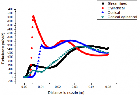
Figure 7. Flow field center turbulent energy curves of the four nozzles
As can be seen from Figure 7, the streamlined nozzle and conical-cylindrical nozzle had relatively small (<1,600m2/s2) turbulent energies on the centerline of the flow field; the energy level changed gently and minimized at the center. This means the two nozzles have a small friction internally and a strong ability to reduce the specific energy of jet. The smallest turbulent energy was observed in the conical nozzle and the front segment of the cylindrical nozzle. This is because the two nozzles have no flow before the sudden change of flow path. In cylindrical nozzle, the turbulent energy jumped to the peak value of 3,055m2/s2 at the sudden change, several times that of the other three nozzles. Hence, the cylindrical nozzle consumed the highest amount of energy, resulting in the highest specific energy of the water jet.
In summary, the streamlined nozzle has the best jet intensity, lowest jet specific energy, highest peak velocity, and longest impact distance among all nozzles. Therefore, this nozzle should be given priority in actual applications. The conical-cylindrical nozzle is the second-best nozzle. Furthermore, the nozzles should be selected according to the specific purpose of the jetting devices. For example, the cutting operation requires fast acceleration and high jet density. Then, streamlined nozzle and conical-cylindrical nozzle should be adopted rather than conical or cylindrical nozzle. For other operations, the nozzles should be selected after comprehensive consideration of the requirements on nozzle performance.
(1) The streamlined nozzle achieved the highest flow velocity and lowest turbulent energy at the centerline of the flow field. This nozzle should be prioritized in actual applications. Meanwhile, conical-cylindrical nozzle strikes a good balance between efficiency and cost, providing a good option for jetting operations. By contrast, conical nozzle and cylindrical nozzle should not be adopted, owing to their high jet density and energy consumption.
(2) During jet acceleration, the jet velocity and intensity in the nozzle are mainly affected by the shape change of the flow path and the stabilizing effect of the cylindrical segment. In the streamlined nozzle, the flow path is changed gently, which contributes to energy conversion and improves jet specific energy. The cylindrical segment can stabilize the shape of the jet by increasing the jet acceleration and peak velocity. The energy consumed in this segment is negligible.
(3) The energy of high-pressure jet is converted in several phases: from electrical or chemical energy to mechanical energy, from mechanical energy to jet energy, from jet energy to kinetic energy, and from kinetic energy to internal energy. The nozzle structure should be optimized to reduce the energy loss in each phase, thereby lowering the energy required to destroy a unit volume of the target, i.e. the specific energy of the jetting device.
The simulation results will be verified through experiments in the future research.
This work was supported by National Key Research and Development Project of China (2017YFC0806608); Natural Science Foundation of Chongqing (cstc2019jcyjmsxmX0286); Youth Fund of Army Logistics College (LQ-QN-201828).
[1] Anwar, S., Axinte, D.A., Becker, A.A. (2013). Finite element modelling of overlapping abrasive waterjet milled footprints. Wear, 303(1-2): 426-436. https://doi.org/10.1016/j.wear.2013.03.018
[2] Deng, J. (2009). Wear behaviors of ceramic nozzles with laminated structure at their entry. Wear, 266(1-2): 30-36. http://dx.doi.org/10.1016/j.wear.2008.05.012
[3] Anwar, S., Axinte, D.A., Becker, A.A. (2013). Finite element modelling of abrasive waterjet milled footprints. Journal of Materials Processing Technology, 213: 180-193. http://dx.doi.org/10.1016/j.jmatprotec.2012.09.006
[4] Durán-Grados, V., Mejías, J., Musina, L., Moreno-Gutiérrez, J. (2018). The influence of the waterjet propulsion system on the ships' energy consumption and emissions inventories. Science of The Total Environment, 631-632(8): 496-509. https://doi.org/10.1016/j.scitotenv.2018.02.291
[5] Schwartzentruber, J., Spelt, J.K. Papini, M. (2017). Prediction of surface roughness in abrasive waterjet trimming of fiber reinforced polymer composites. International Journal of Machine Tools and Manufacture, 122(11): 1-17. https://doi.org/10.1016/j.ijmachtools.2017.05.007
[6] Zeidan, D., Zhang, L., Goncalves, E. (2018). Cavitating bubbly flow computations by means of mixture balance equations. 3rd Thermal and Fluids Engineering Conference, 2018: 1681-1687. http://dx.doi.org/10.1615/TFEC2018.mph.021541
[7] Ahmed, T.M., Mesalamy, A.S.E., Youssef, A., Midany, T.T.E. (2018). Improving surface roughness of abrasive waterjet cutting process by using statistical modeling. CIRP Journal of Manufacturing Science and Technology, 22(8): 30-36. https://doi.org/10.1016/j.cirpj.2018.03.004
[8] Nie, B.S., Wang, H., Li, L., Zhang, J.F., Yang, H., Liu Z., Wang, L.K., Li, H.L. (2011). Numerical investigation of the flow field inside and outside high-pressure abrasive waterjet nozzle. Procedia Engineering, 26(12): 48-55. https://doi.org/10.1016/j.proeng.2011.11.2138
[9] Pozzetti, G., Peters, B. (2018). A numerical approach for the evaluation of particle-induced erosion in an abrasive waterjet focusing tube. Powder Technology, 333(6): 229-242. https://doi.org/10.1016/j.powtec.2018.04.006
[10] Li, D., Kang, Y., Ding, X.L., Wang, X.C., Fang, Z.L. (2016). Effects of area discontinuity at nozzle inlet on the characteristics of self-resonating cavitating waterjet. Chinese Journal of Mechanical Engineering, 29(4): 813-823. http://dx.doi.org/10.3901/CJME.2016.0426.060
[11] Kizaki, A., Ishii, H., Imai, T. (2017). Waterjet drilling of sealing cement. Procedia Engineering, 191: 869-872. https://doi.org/10.1016/j.proeng.2017.05.255
[12] Barsukov, G., Zhuravleva, T., Kozhus, O. (2017). Quality of hydroabrasive waterjet cutting machinability. Procedia Engineering, 206: 1034-1038. https://doi.org/10.1016/j.proeng.2017.10.590
[13] Mieszala, M., Lozano Torrubia, P., Axinte, D.A., Schwiedrzik, J.J., Guo, Y., Mischler, S., Michler, J., Philippe, L. (2017). Erosion mechanisms during abrasive waterjet machining: Model microstructures and single particle experiments. Journal of Materials Processing Technology, 247(9): 92-102. https://doi.org/10.1016/j.jmatprotec.2017.04.003
[14] Flynn, M.A., Wang, A.Y. (2014). Underwater endoscopic mucosal resection of large duodenal adenomas (video). Video Journal and Encyclopedia of GI Endoscopy, 2(3-4): 84-86. https://doi.org/10.1016/j.vjgien.2015.02.002
[15] Kizaki, A., Ishii, H., Imai, T. (2017). Waterjet drilling of sealing cement. Procedia Engineering, 191: 869-872. https://doi.org/10.1016/j.proeng.2017.05.255
[16] Alberdi, A., Rivero, A., Artaza, T., Lamikiz, A. (2017). Analysis of alloy 718 surfaces milled by abrasive waterjet and post-processed by plain waterjet technology. Procedia Manufacturing, 13: 679-686. https://doi.org/10.1016/j.promfg.2017.09.163
[17] Uhlmann, E., Flögel, K., Sammler, F., Rieck, I., Dethlefs, A. (2014). Machining of hypereutectic aluminum silicon alloys. Procedia CIRP, 14(7): 223-228. https://doi.org/10.1016/j.procir.2014.03.069
[18] Ozcelik, Y., Tercan, A.E., Yilmazkaya, E., Ciccu, R., Costa, G. (2011). A study of nozzle angle in stone surface treatment with water jets. Construction and Building Materials, 25(11): 4271-4278. http://dx.doi.org/10.1016/j.conbuildmat.2011.04.071
[19] Wang, Y.F., Zhang, Z., Zhang, G.Y., Wang, B. Zhang, W.W. (2017). Study on immersion waterjet assisted laser micromachining process. Journal of Materials Processing Technology, 262(12): 290-298. https://doi.org/10.1016/j.jmatprotec.2018.07.004
[20] Nouraei, H., Kowsari, K., Spelt, J.K., Papini, M. (2014). Surface evolution models for abrasive slurry jet micro-machining of channels and holes in glass. Wear, 309(1-2): 65-73. https://doi.org/10.1016/j.wear.2013.11.003
[21] Matsumura, T., Muramatsu, T., Fueki, S. (2011). Abrasive water jet machining of glass with stagnation effect. CIRP Annals, 60(1): 355-358. https://doi.org/10.1016/j.cirp.2011.03.118
[22] Eslamdoost, A., Larsson, L., Bensow, R. (2018). Analysis of the thrust deduction in waterjet propulsion – The Froude number dependence. Ocean Engineering, 152(5): 100-112. https://doi.org/10.1016/j.oceaneng.2018.01.037
[23] Gent, M., Menéndez, M., Torno, S., Toraño, J., Schenk, A. (2012). Experimental evaluation of the physical properties required of abrasives for optimizing waterjet cutting of ductile materials. Wear, 284-285: 43-51. http://dx.doi.org/10.1016/j.wear.2012.02.012
[24] Wu, X.J., Choi, J.K., Singh, S., Hsiao, C.T., Chahine, G.L. (2012). Experimental and numerical investigation of bubble augmented waterjet propulsion. Journal of Hydrodynamics, 24(5): 635-647. http://dx.doi.org/10.1016/S1001-6058(11)60287-4
[25] Viganò, F., Cristiani, C., Annoni, M. (2017). Ceramic sponge Abrasive Waterjet (AWJ) precision cutting through a temporary filling procedure. Journal of Manufacturing Processes, 28(8): 41-49. https://doi.org/10.1016/j.jmapro.2017.05.014