Zhixian Ye* | Yang Zhang | Jianfeng Zou | Yao Zheng
OPEN ACCESS
This paper installs a zero-pressure gradient measurement platform in a low velocity wind tunnel. A smooth plate and four riblet plates were designed and tested on the platform. A constant-temperature hot-wire anemometer (HWA) was adopted to measure the velocity distribution in the turbulent boundary layer above each plate to detect the effect of riblet structures on the near-wall turbulence. The mean velocity distribution of the boundary layer was fitted, using Spalding’s “law of the wall” (LW) formula and least squares (LS) method, to get the friction velocity and frictional stress on the wall. And the high-order turbulence statistics, autocorrelation coefficients and energy spectrum curves are calculated to compare the drag reduction features of different riblet structures. The results show that the riblet structure could restrict the spanwise flow at the bottom of the boundary layer, and reduce the drag by 10% in local areas; with suitable parameters, the sinusoidal riblet, which is arranged in the streamwise direction, has greater drag reduction than the straight riblets. This is because the sinusoidal riblet could induce orderly spanwise motions at the bottom, similar to spanwise vibrations, making the spanwise velocity distribution at the bottom more orderly.
tunnel measurement, riblet surface, turbulent boundary layer, hot-wire anemometer (HWA), drag reduction
In the 1970s, NASA’s Langley Research Center found that the streamwise small riblets on the surface of an object can effectively suppress the frictional drag on turbulent wall. This finding goes against the traditional view that the drag is negatively correlated with surface smoothness. Since then, riblet drag reduction has been widely considered to reduce the drag of turbulence structure [1].
Walsh et al. [2-5] from NASA’s Langley Research Center probed deep into riblet drag reduction, pointing out that the symmetric V-riblet surface can effectively reduce the drag, if the dimensionless height is 25 and the dimensionless interval is 30. After measuring the velocity distribution, Bacher and Smith [6] reduced the drag by 25% with riblets, using the boundary-layer momentum integral equation. Gallagher and Thomas [7] also used the boundary-layer momentum integral equation to calculate the effect of riblet drag reduction, and concluded that drag is only reduced in the latter half of the riblet plate, while the total drag remains basically unchanged. Park and Wallace [8] adopted a hot-wire anemometer (HWA) to measure the streamwise velocity field of riblet surface, and reduced about 4% of the drag by integrating the frictional shear stress on the riblet wall. Bechert [9] reduced the drag by 9.9% on a height-adjustable thin-blade riblet surface, suggesting that the best drag reduction geometry is the thin-blade riblet surface with a suitable aspect ratio. Because the thin-blade riblet is very complex to fabricate, most studies on riblet drag reduction focus on the traditional symmetric V-riblet surface. Some scholars have explored the riblets that are curved in the streamwise direction. Through large eddy simulation, Peet and Sagaut [10] observed that the sinusoidal riblet reduced the drag by 7.4%, 50% higher than that (5.4%) of the straight riblet under the same conditions. Miki [11] designed a Z-riblet whose lateral spacing expands and contracts in the linear direction, and achieved the total drag reduction of 9%, including 23% decrease of surface frictional drag and 14% increase of pressure drag. Sasamori et al. [12] measured the drag reduction of a sinusoidal riblet with a particle image velocimeter (PIV), revealing that the riblet could reduce 11.7% of the drag at the most. Kramer [13] held that the curved riblet outperforms the straight riblet in drag reduction, because it can induce regular spanwise motions at the bottom of the boundary layer, similar to how the spanwise vibrations of the flat plate on the turbulence structure; under the regular spanwise motions, the disordered distribution of spanwise velocity on the boundary layer will become more orderly.
Riblet drag reduction have been applied to aircrafts, flow-driven equipment, etc. For instance, the Airbus [14] covered 70% of the surface of an A320 prototype with a riblet film, saving about 1~2% of fuel. NASA’s Langley Research Center [15, 16] tested that the riblet film reduced roughly 6% of the surface drag of Learjet. The Fastskin swimsuits of Speedo International Ltd. [17] can lower the water drag by 2%. KSB [18], a world’s leading manufacturers of pumps and valves, machined regular riblets on the blades of multi-stage pumps, and thus increased the overall pumping efficiency by 1.5%. And some apparatuses have been adopted to measure the riblet drag reduction in microfluidic structures, such as the PIV, the HWA and the Laser Doppler Velocimeter (LDV). Unlike force balance or other devices that directly measure the drag, these flow field measuring apparatuses capture the drag reduction effect indirectly after measuring the characteristic parameters of near-wall flow field of the riblet structure, computing the friction velocity on the wall, and acquiring the local frictional drags. Anthony Kendall et al. [19] estimated the wall friction in turbulent wall-bounded flow, using the Musker profile and the Spalding profile. Hooshand et al. used the Clauser [20] chart method to obtain the friction velocity, and highlighted the necessity to measure the velocity distribution accurately within the boundary layers (i.e. the viscous sublayer and the logarithmic layer) before computing the friction velocity by Spalding’s “law of the wall” (LW) formula.
In this paper, a zero-pressure gradient platform is set up in a low-velocity wind tunnel. Then, a constant-temperature HWA was adopted to measure the flow field information of a smooth plate and four riblet plates of different sizes. Based on the velocity distribution in the turbulent boundary layer, the friction velocities of different plates were fitted by Spalding’s LW formula and the least squares (LS) method, reflecting the difference between the riblet structures in frictional stress. In addition, the drag reduction effects of different riblet surfaces on the turbulent boundary layer were evaluated comprehensively through high-order statistical analysis, autocorrelation analysis and energy spectrum analysis.
2.1 Test instruments
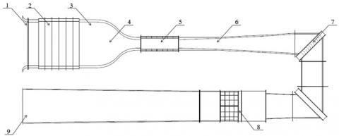
As shown in Figure 1, the test site is a low-turbulence, low-velocity, open-jet wind tunnel of the School of Aeronautics and Astronautics, Zhejiang University, China. The test section is 3.5m-long, 1.2m-wide and 1.2m-tall. The maximum wind velocity was set to 70m/s, and the turbulence coefficient to 0.04~0.05 %. The test data were collected by a StreamLine constant-temperature HWA (Dantec Dynamics, Denmark). The data in the turbulent boundary layer were collected by a 55P15 boundary layer probe, which contains a single straight wire. To control the spatial positions of the measuring points, the probe was installed on a displacement guide rail on the top of the test section. The turbulent boundary layers of a smooth plate and several riblet plates were measured and analyzed to disclose their flow field features.
1. Tunnel inlet 2. Deflector nets 3. Stable section 4. Contraction section 5. Test section 6. Diffuser section 7. Corner 8. Engine section 9. Tunnel outlet
Figure 1. The wind tunnels
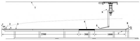
The 4m-long, 1m-wide test platform was stitched up from four acrylic plates. The acrylic plates were supported by an aluminum alloy frame, keeping the plate joints are flat and level. In addition, 20cm-tall vertical acrylic plates were installed on both sides of the platform, aiming to eliminate the wall effect on the flow field. To keep the pressure gradient of the platform at zero, an adjustable inclination tail board was installed on the rear edge of the platform. Meanwhile, a 40mm-wide emery belt and a trip wire were applied on the wedge-shaped leading edge for manual turning. To facilitate the replacement of test plates, a 50×50 cm mounting hole was opened at 250~300 cm right ahead of the center of the leading edge of the platform. In the mounting hole, a high-precision displacement lifting table was provided to keep the plate edge on the same level with the platform surface. The right-handed coordinate system was adopted, with the origin at the intersection of the leading-edge line and the symmetry plane, the x-axis along the stream, the y-axis along the normal direction and the z-axis along the span direction. The test platform is described in Figure 2 below.
1. Wind tunnel wall 2. Tripping tape 3. Test plate 4. Synthetic jet array 5. Hot wire probe 6. Guide rail 7. Support 8. Tail board
Figure 2. The test platform
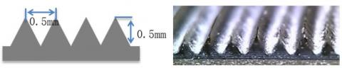
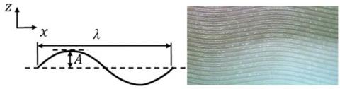
The test objects include a smooth plate and four riblet plates. Each riblet plate is 10mm-thick, and was milled from 500×500mm acrylic plate. As shown in Figure 3, the cross-section of the riblet structure is an isosceles triangle, where both the bottom width s and height hare 0.5 mm. As mentioned before, four different riblet plates were prepared. The first riblet plate has straight riblets with h=s=0.5 mm. The second riblet plate has sinusoidal riblets with h=s=0.5 mm, streamwise wavelength λ=30 mm and amplitude A=1 mm. The third riblet plate has sinusoidal riblets with h=s=0.5 mm, streamwise wavelength λ=30 mm and amplitude A=2 mm. The fourth riblet plate has sinusoidal riblets with h=s=0.5mm, streamwise wavelength λ=30 mm and amplitude A=3 mm. The sinusoidal riblets are illustrated in Figure 4. Table 1 lists the serial number of each test plate.
Figure 3. Riblet cross-section
Figure 4. Sinusoidal riblets
Table 1. Serial number of each test plate
|
Serial number |
A |
|
#1 |
smooth |
|
#2 |
0 mm, straight |
|
#3 |
1 mm, sinusoidal |
|
#4 |
2 mm, sinusoidal |
|
#5 |
3 mm, sinusoidal |
2.2 Measurement methods
The riblet channels were placed along the streamwise direction. The vertical distribution of mean flow velocity of smooth surface and riblet surfaces were measured at the same position. The HWA was used to measure the center point of the test plate, i.e. 275 cm in the front of the leading edge of the test platform and on the centerline in the width direction of the tunnel.
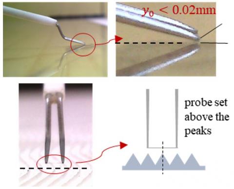
During the tests, the probe position was controlled by the displacement guide rail. To eliminate the travel error, the flow velocity was measured continuously across the plate surface from near too far. The start position was close enough to but not in contact with the plate. A digital microscope was adopted to monitor how the probe approaches the plate. In the vertical direction, the probe position could be adjusted by 0.01 mm at the least at a time. The distance between the start position and the test plate (Figure 5) was evaluated based on the measured results of the digital microscope, and used for parameter fitting by Spalding’s LW formula.
From the plate surface (or the top of the riblet structure for riblet plates) to the outmost layer of the turbulent boundary layer, 64 measuring points were arranged on each plate with unequal intervals. The HWA collected data at the frequency of 64 kHz. The sampling lasts 30 s at each measuring point. A total of 1,920,000 sample points was collected. During the tests, the flow velocity in the tunnel was 15 m/s.
Figure 5. The start position of measurement
2.3 Calculation method of frictional stress
In general, the turbulent boundary layer can be divided into a viscous sublayer, a buffer layer, a logarithmic layer and an outer layer. In the viscous sublayer, the dominant force is viscous friction, and the velocity distribution is $u^{+}=y^{+}$; in the logarithmic layer, the dominant force is turbulent shear stress (Reynolds stress), and the velocity distribution is $u^{+}=\ln y^{+} / \kappa+B$. Note that $u^{+}=u / u_{\tau}$ and $y^{+}=y u_{\tau} / v$, where y is the vertical height, u is the time-averaged velocity, $u_{\tau}$ is the friction velocity, ν is the kinematic viscosity; κ is the von Kármán constant; B is the integration constant; $u^{+}$ and $y^+$ are dimensionless velocity and wall distance, respectively.
The viscous sublayer is very close to the wall, making it difficult to measure. The Clauser chart method was often adopted to evaluate the frictional stress on the wall $u_τ$. By this method, the $u_τ$ is fitted based on the velocity distribution in the logarithmic layer, and then the frictional stress on the wall can be estimated by $u_{\tau} \equiv \sqrt{\tau_{w} / \rho}$. There are two major limitations of this method: The data range of the logarithmic layer is selected rather subjectively, without including the data points near the wall; The method tends to exaggerate the friction velocity [21]. To overcome the limitations, the Spalding’s LW formula [22] is selected for this research. This is a power series interpolation formula that considers all the area from the viscous sublayer to the logarithmic layer:
$y^{+}=u^{+}+e^{-\kappa B}\left[e^{\kappa u^{+}}-1-\kappa u^{+}-\frac{\left(\kappa u^{+}\right)^{2}}{2}-\frac{\left(\kappa u^{+}\right)^{3}}{6}\right]$
$y^{+}=\frac{\left(y+y_{0}\right) u_{\tau}}{v}, u^{+}=\frac{u}{u_{\tau}}$
where, y0 is the virtual origin. The other parameters have the same meanings as above.
3.1 Velocity profiles of boundary layer
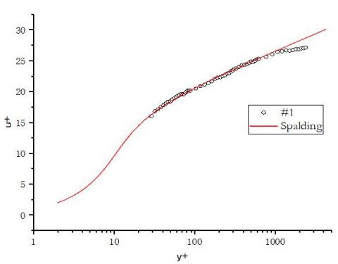
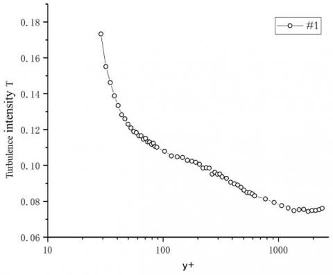
Firstly, the time-averaged velocity profile of the smooth plate #1 was fitted. The resulting time-averaged velocity and turbulence intensity T are displayed in Figures 6, respectively. The turbulence intensity T was introduced to characterize the fluctuating degree of the pulsation velocity u':
$\mathrm{T}=\frac{\sqrt{<u^{\prime 2}>}}{u}$
Four parameters were obtained through the parameter fitting, namely, the virtual origin y0, the friction velocity $u_τ$, the von Kármán constant κ and the integration constant B. The von Kármán constant κ is generally believed to be closely related to the test conditions. Therefore, the κ value was kept the same for the parameter fitting of all test plates. In other words, the parameter fitting of any other test plate only needs to determine the values of the virtual origin y0, the friction velocity $u_τ$, and the integration constant B.
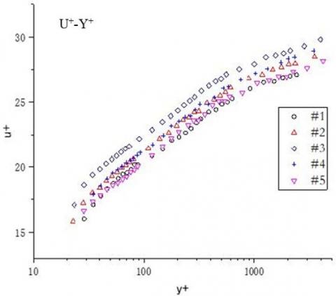
Figure 7 shows the time-averaged velocity profile and turbulence intensity of each plate, which was drawn based on the dimensionless friction velocity of the corresponding plate. The curves of the riblet plates were higher than the curve of the smooth plate, indicating that the flow velocities of the riblet plates are greater than the flow velocity at the same position of the smooth plate. The results demonstrate the drag reduction effects of the riblet plates.
As shown in Figures 6 and 7, the turbulence intensity T did not decrease in the place next to the wall, i.e. at a small dimensionless wall distance $y^+$. This means the probe has not reached the viscous sub-layer. In near-wall region, riblet plates #2, #3, #4 and #5 saw different degrees of decline in turbulence intensity from the level of smooth plate #1. The decline reflects that the disordered spanwise flow is restricted by the riblets and becomes more orderly.
Table 2. The main parameters of the test plates
|
Serial number |
κ |
$\boldsymbol{u}_{\boldsymbol{\tau}} / \mathbf{m} \cdot \mathbf{s}^{-1}$ |
B |
y0/mm |
Drag reduction |
|
#1 |
0.4139 |
0.5350 |
9.846 |
0.9760 |
/ |
|
#2 |
0.5217 |
10.720 |
0.7844 |
4.91% |
|
|
#3 |
0.5043 |
11.290 |
0.7311 |
11.15% |
|
|
#4 |
0.5135 |
10.920 |
1.2350 |
7.88% |
|
|
#5 |
0.5340 |
10.090 |
0.9679 |
0.37% |
Figure 6. Time-averaged velocity profile and turbulence intensity of the smooth plate
Figure 7. Time-averaged velocity profile and turbulence intensity of each plate
3.3 High-order statistical analysis
The measured velocity is superimposed by the average velocity and the pulsation velocity, and can thus be considered a stochastic stationary signal. To disclose the variation in the statistical features of the pulsation velocity from place to place, it is necessary to analyze the high-order statistics of the pulsation velocity.
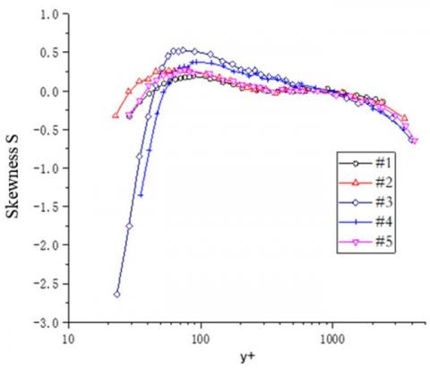
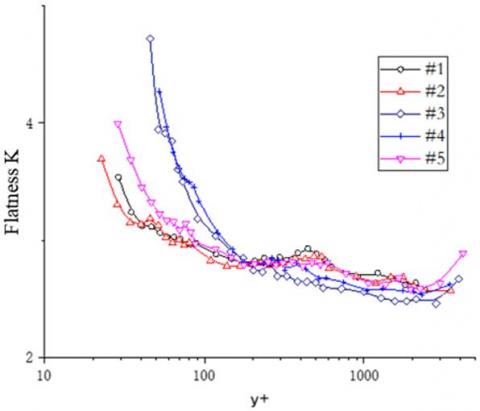
Two statistics were selected to analyze the turbulence, including skewness S and flatness K. The former reflects the non-uniformity of the probability density distribution of the pulsation velocity, and the latter showcases the intermittency of the turbulence. The skewness S and flatness K can be respectively computed by:
$S=\frac{<u^{\prime 3}>}{\left(<u^{\prime 2}>\right)^{3 / 2}}=\frac{\frac{1}{N} \sum_{i=1}^{N} u_{i}^{\prime 3}}{\left(\frac{1}{N} \sum_{i=1}^{N} u_{i}^{\prime 2}\right)^{\frac{3}{2}}}$
$\mathrm{K}=\frac{<u^{\prime 4}>}{\left(<u^{\prime 2}>\right)^{2}}=\frac{\frac{1}{N} \sum_{i=1}^{N} u_{i}^{\prime 4}}{\left(\frac{1}{N} \sum_{i=1}^{N} u_{i}^{\prime 2}\right)^{2}}$
where, u' is the pulsation velocity; N is the number of data points.
Figures 8 presents the skewness profile and flatness profile of each plate, respectively. It can be seen that, in the near-wall region, the riblet plates #3 and #4 had way smaller skewness but much higher flatness than plates #1 and #2.
Figure 8. Skewness profile and flatness profile of each plate
3.3 Autocorrelation analysis
Correlation analysis is an important means to characterize turbulence structure. It helps to disclose the correlations between flow elements in time, space and spacetime. In this paper, the most basic way of correlation analysis, i.e. autocorrelation analysis of time series, is selected to discuss the drag reduction effects of different plates. Under the premise that the turbulence velocity is a stochastic stationary signal with ergodicity, the autocorrelation functions were set up as follows for the pulsation velocities at the same position of different plates:
$\mathrm{R}(\mathrm{n})=\frac{\sum_{i=n+1}^{N} u^{\prime}(i) \cdot u^{\prime}(i-n)}{u_{r m s}^{\prime 2}}$
where, n is the time interval; N is the number of data points; $u_{r m s}^{\prime 2}$ is the variance of the pulsation velocity.
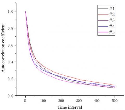
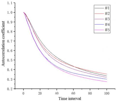
Figure 9. Autocorrelation coefficients (time interval: 0~500 and 0~100)
The decrement (increment) of the autocorrelation coefficient means the scale of the integral time, which is defined by the integration from the origin to the infinity, is decreasing (increasing). This scale directly reflects the scale of the turbulence structure [19]. If the turbulence is completely disordered, i.e. similar to white noise, the autocorrelation was zero, and the turbulence structure is small; if the turbulence is completely free of fluctuations, i.e. almost constant, the autocorrelation is one, and the turbulence structure is large.
Figures 9 displays the autocorrelation coefficients of pulsation velocity at the bottom of each plate under different time intervals. It can be seen that riblet plates #2~#5 had smaller autocorrelation coefficient than the smooth plate #1 under the short time interval. With the growth in the time interval, the autocorrelation coefficient of each riblet plate was on the rise, as evidenced by the increased slope of the curve. The sinusoidal riblet plates #3~5 witnessed greater increase of the autocorrelation coefficient than the straight riblet plate #2. Among the sinusoidal riblet plates, the autocorrelation coefficient increased more markedly for the plate with relatively large amplitude.
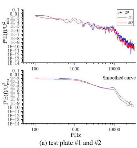
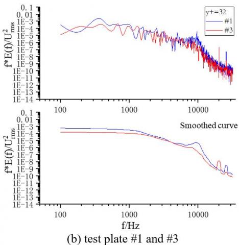
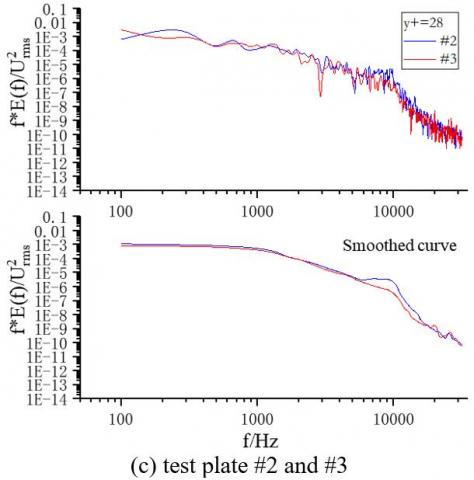
3.4 Energy spectrum analysis
The energy spectrum curve of each plate was plotted based on the dimensionless pulsation velocity. This curve expresses how much the fluctuation frequency of velocity contributes to the kinetic energy of the turbulence, and helps to piece up the basic condition of the turbulent flow field. In an energy spectrum curve, the low-frequency part is the generation region, in which the kinetic energy is produced by buoyancy and shearing; the medium-frequency part is the dissipation region, in which the kinetic energy is converted to internal energy due to viscosity; the high-frequency part is the inertia region, in which the kinetic energy is neither produced nor dissipated, but continuously transmitted to small-scale areas.
Figure 10. Energy spectrum curves of different test plates
From Figures 10, it can be seen that, when the dimensionless wall distance y+ was the same, the energy spectrum curve of either straight riblet plate #2 or sinusoidal riblet plate #3 was below that of smooth plate #1, in both the dissipation region and the generation region; the energy spectrum curve of sinusoidal riblet plate #3 was lower than that of straight riblet plate #2. These phenomena manifest that the riblets reduce the energy loss, and sinusoidal riblet is more energy efficient than straight riblet. These findings agree with the previous analysis on drag reduction effects.
This paper installs a zero-pressure gradient measurement platform in a low-velocity wind tunnel. Next, an HWA was adopted to measure the velocity distribution in the boundary layer of wall turbulence. Based on the measured results, the author discussed how different riblet structures affect the turbulence and reduce the drag on the wall. The following conclusions were drawn through the research:
(1) For the wall turbulence, adding a riblet structure to the boundary layer helps to lift the velocity distribution in the boundary layer and reduce the frictional drag; if the riblets are of the same cross-sectional shape, the sinusoidal riblet ($A^{+}=25, \lambda^{+}=700$) arranged in the streamwise direction can reduce the drag more effectively than the straight riblet. However, the drag reduction effect decreases with the amplitude of the sinusoidal curve.
(2) In the near-wall region, the riblet plates had way smaller skewness but much higher flatness than plates. The autocorrelation coefficients of the riblet plates were on the rise, as the short time interval gradually increased. This means the riblets could restrict the spanwise disordered flow at the bottom of the boundary layer, while producing regular slow spanwise movements.
(3) At the same height, the energy spectrum curve of each riblet plate, which has the drag reduction effect, was lower than that of the smooth plate; the energy spectrum curve of a typical sinusoidal riblet was below that of the straight riblet plate. These phenomena show that the riblet structure can regulate the flow in the boundary layer, and that the sinusoidal riblet has greater ability than the straight riblet to make the velocity distribution in the boundary layer more orderly.
The authors would like to acknowledge the financial support received from the project “Drag Reduction via Turbulent Boundary Layer Flow Control (DRAGY)”. The DRAGY project (April 2016 - March 2019) is a China-EU Aeronautical Cooperation project, which is co-funded by Ministry of Industry and Information Technology (MIIT), China, and Directorate-General for Research and Innovation (DG RTD), European Commission.
[1] Bechert, D.W., Bruse, M., Hage, W., Meyer, R. (2000). Fluid mechanics of biological surfaces and their technological application. Naturwissenschaften, 87(4): 157-171. https://doi.org/10.1007/s001140050696
[2] Walsh, M.J. (1983). Riblets as a viscous drag reduction technique. AIAA Journal, 21(4): 485-486. https://doi.org/10.2514/3.60126
[3] Walsh, M. (1982). Turbulent boundary layer drag reduction using riblets. 20th Aerospace Sciences Meeting, pp. 169-169. https://doi.org/10.2514/6.1982-169
[4] Walsh, M., Lindemann, A. (1984). Optimization and application of riblets for turbulent drag reduction. 22nd Aerospace Sciences Meeting, pp. 347-347. https://doi.org/10.2514/6.1984-347
[5] Walsh, M.J. (1990). Viscous drag reduction in boundary layers. Riblets, pp. 203-261. https://doi.org/10.2514/5.9781600865978.0203.0261
[6] Bacher, E.V., Smith, C.R. (1985). A combined visualization-anemometry study of the turbulent drag reducing mechanisms of triangular micro-groove surface modifications. Shear Flow Control Conference, 85-548. https://doi.org/10.2514/6.1985-548
[7] Gallagher, J., Thomas, A. (1984). Turbulent boundary layer characteristics over streamwise grooves. 2nd Applied Aerodynamics Conference, pp. 1984-2185. https://doi.org/10.2514/6.1984-2185
[8] Park, S.R., Wallace, J.M. (1994). Flow alteration and drag reduction by riblets in a turbulent boundary layer. AIAA Journal, 32(1): 31-38. https://doi.org/10.2514/3.11947
[9] Bechert, D.W., Bruse, M., Hage, W, van der Hoeven, J.G.T. (1997). Experiments on drag-reducing surfaces and their optimization with an adjustable geometry. Journal of Fluid Mechanics, 338: 59-87. https://doi.org/10.1017/S0022112096004673
[10] Peet, Y., Sagaut, P., Charron, Y. (2008). Turbulent drag reduction using sinusoidal riblets with triangular cross-section. 38th Fluid Dynamics Conference and Exhibit, 3745(23-26): 1-9. https://doi.org/10.2514/6.2008-3745
[11] Miki, H., Iwamoto, K., Murata, A. (2011). PIV analysis on a 3-dimensional riblet for drag reduction. Transactions of the Japan Society of Mechanical Engineers, Series B, 77(782): 25-36. https://doi.org/10.1299/kikaib.77.1892
[12] Sasamori, M., Mamori, H., Iwamoto, K., Murata, A. (2014). Experimental study on drag-reduction effect due to sinusoidal riblets in turbulent channel flow. Experiments in Fluids, 55(10): 1828-1828. https://doi.org/10.1007/s00348-014-1828-z
[13] Kramer, F., Grueneberger, R., Thiele, F.H., Wassen, E. Wavy riblets for turbulent drag reduction. 5th Flow Control Conference, 4583: 1-10. https://doi.org/10.2514/6.2010-4583
[14] Szodruch, J. (1991). Viscous drag reduction on transport aircraft. 29th Aerospace Sciences Meeting, pp. 91-685. https://doi.org/10.2514/6.1991-685
[15] Bechert, D., Reif, W. (1985). On the drag reduction of the shark skin. 23rd Aerospace Sciences Meeting, pp. 546-546. https://doi.org/10.2514/6.1985-546
[16] Bacher, E., Smith, C. (1985). A combined visualization-anemometry study of the turbulent drag reducing mechanisms of triangular micro-groove surface modifications. Shear Flow Control Conference, pp. 548-548. https://doi.org/10.2514/6.1985-548
[17] Toussaint, H.M., Truijens, M., Elzinga, M.J, van de Ven, A., de Best, H., Snabel, B., de Groot, G. (2002). Effect of a Fast-skin 'body' suit on drag during front crawl swimming. Sports Biomechanics, 1(1): 1-10. https://doi.org/10.1080/14763140208522783
[18] Pauly, C.P. (2001). What is a shark doing in this pump. World Pumps, (423): 15-16. https://doi.org/10.1016/S0262-1762(01)80387-4
[19] Kendall, A., Koochesfahani, M. (2006). A method for estimating wall friction in turbulent boundary layers. 25th AIAA Aerodynamic Measurement Technology and Ground Testing Conference, 3834: 1-6. https://doi.org/10.2514/6.2006-3834
[20] Clauser, F.H. (1956). The turbulent boundary layer. Advances in Applied Mechanics. Elsevier, 4: 1-51. https://doi.org/10.1016/S0065-2156(08)70370-3
[21] Kendall, A., Koochesfahani, M. (2008). A method for estimating wall friction in turbulent wall-bounded flows. Experiments in Fluids, 44(5): 773-780. https://doi.org/10.1007/s00348-007-0433-9
[22] Spalding, D.B. (1961). A single formula for the "law of the wall". Journal of Applied Mechanics, 28(3): 455-458. https://doi.org/10.1115/1.3641728